Chapter 3 SCPME
In their 2017 paper, titled Shrinking Characteristics of Precision Matrix Estimators, Aaron Molstad, Ph.D. and Professor Adam Rothman outline a framework to shrink a characteristic of a precision matrix. This concept, inspired by others like Cai and Liu (2011), Fan, Feng, and Tong (2012), and Mai, Zou, and Yuan (2012), exploits the fact that in many predictive models estimation of the precision matrix is only necessary through its product with another feature, such as a mean vector. The example they offer in Molstad and Rothman (2017) is in the context of Fisher’s linear discriminant analysis model. If a response vector \(Y\) is categorical such that \(Y\) can take values in \(\left\{1, ..., J\right\}\), then the linear discrimnant analysis model assumes that the predictor matrix \(X\) conditional on the response vector \(Y\) is normally distributed:
\[\begin{equation} X | Y = j \sim N_{p}\left(\mu_{j}, \Omega^{-1}\right) \tag{3.1} \end{equation}\]
for each \(j = 1, ..., J\). One can see from this formulation that clearly an estimation of both \(\mu\) and \(\Omega\) are required for this model. However, they note that if prediction is the primary concern, then for a given observation \(X_{i}\) only the characteristic \(\Omega\left(\mu_{l} - \mu_{m}\right)\) is needed to discern between response categories \(l\) and \(m\). In other words, prediction only requires the characteristic \(\Omega\left(\mu_{l} - \mu_{m}\right)\) for each \(l, m \in \left\{1, ..., J\right\}\) and does not require estimation of the full precision matrix \(\Omega\). Cai and Liu (2011) were among the first authors to propose estimating this characteristic directly but the interesting facet that distinguishes Molstad and Rothman’s approach is that their framework simultaneously fits the model in (3.1) and performs variable selection.
The general framework has applications outside of linear discriminant analysis and we will be exploring a regression application in later sections, but first we will outline their approach. The penalty proposed by Molstad and Rothman (2017) is of the form
\[\begin{equation} P\left(\Omega\right) = \lambda\left\| A\Omega B - C \right\|_{1} \tag{3.2} \end{equation}\]
where \(A \in \mathbb{R}^{m \times p}, B \in \mathbb{R}^{p \times q}, \mbox{ and } C \in \mathbb{R}^{m \times q}\) are matrices that are assumed to be known and specified so that solving the full penalized gaussian negative log-likelihood for \(\Omega\) results in solving
\[\begin{equation} \hat{\Omega} = \arg\min_{\Omega \in S_{+}^{p}}\left\{ tr\left(S\Omega\right) - \log\left|\Omega \right| + \lambda\left\| A\Omega B - C \right\|_{1} \right\} \tag{3.3} \end{equation}\]
A similar estimator was proposed by Dalal and Rajaratnam (2017) when \(C = 0\) but here we do not require it. This form of penalty is particularly useful because it is extremely general. Note that by letting matrices \(A = I_{p}, B = I_{p}, \mbox{ and } C = 0\), this penalty reduces to a lasso penalty - but clearly this form allows for much more creative penalties and \(A, B, \mbox{ and } C\) can be constructed so that we penalize the sum, absolute value of many characteristics of the precision matrix \(\Omega\). We will explore how to solve for \(\hat{\Omega}\) in (3.3) in the next section.
3.1 Augmented ADMM Algorithm
Solving for \(\hat{\Omega}\) in (3.3) uses what we are going to call an augmented ADMM algorithm. Molstad and Rothman do not offer a name for this specific algorithm but it leverages the majorize-minimize principle in one of the steps in the algorithm - augmenting the original ADMM algorithm discussed in the previous chapter. Within the context of the proposed penalty, the original ADMM algorithm for precision matrix estimation would consist of iterating over the following three steps:
\[\begin{equation} \begin{split} \Omega^{k + 1} &= \arg\min_{\Omega \in \mathbb{S}_{+}^{p}}L_{\rho}(\Omega, Z^{k}, \Lambda^{k}) \\ Z^{k + 1} &= \arg\min_{Z \in \mathbb{R}^{n \times r}}L_{\rho}(\Omega^{k + 1}, Z, \Lambda^{k}) \\ \Lambda^{k + 1} &= \Lambda^{k} + \rho\left(A\Omega^{k + 1}B - Z^{k + 1} - C \right) \end{split} \tag{3.4} \end{equation}\]
where \(L\), the augmented lagrangian, is defined as
\[\begin{equation} L_{\rho}(\Omega, Z, \Lambda) = f\left(\Omega\right) + g\left(Z\right) + tr\left[\Lambda '\left(A\Omega B - Z - C\right)\right] + \frac{\rho}{2}\left\|A\Omega B - Z - C\right\|_{F}^{2} \tag{3.5} \end{equation}\]
Similar to the previous chapter, \(f\left(\Omega\right) = tr\left(S\Omega\right) - \log\left|\Omega\right|\) and \(g\left(Z\right) = \lambda\left\|Z\right\|_{1}\). In fact, the details of the algorithm thus far are identical to the previous approach except that we are replacing \(\Omega - Z\) with \(A\Omega B - Z - C\) in the augmented lagrangian and the dual update \(\Lambda^{k + 1}\).
Instead of solving the first step directly, the authors propose an alternative, approximating objective function, which we will denote as \(\tilde{L}\), that is based on the majorize-minimize principle5. The purpose of this approximating function is the desire to solve the first step of the algorithm in closed-form. The ADMM algorithm with this modification based on majorize-minimize principle is also found in Lange (2016) but here we define the approximating function as
\[\begin{equation} \begin{split} \tilde{L}_{\rho}\left(\Omega, Z^{k}, \Lambda^{k}\right) = f\left(\Omega\right) &+ g\left(Z^{k}\right) + tr\left[(\Lambda^{k})'(A\Omega B - Z^{k} - C) \right] + \frac{\rho}{2}\left\|A\Omega B - Z^{k} - C \right\|_{F}^{2} \\ &+ \frac{\rho}{2}vec\left(\Omega - \Omega^{k}\right)' Q\left(\Omega - \Omega^{k}\right) \end{split} \tag{3.6} \end{equation}\]
where \(Q = \tau I_{p} - \left(A'A \otimes BB'\right)\) and \(\tau\) is chosen such that \(Q\) is positive definite. Note that if \(Q\) is positive definite, then \(L_{\rho}\left(\cdot\right) \leq \tilde{L}\left(\cdot\right)\) for all \(\Omega\) and \(\tilde{L}\) is a majorizing function6. The augmented ADMM algorithm developed by Molstad and Rothman, which now includes the majorize-minimize principle, consists of the following repeated iterations:
\[\begin{equation} \begin{split} \Omega^{k + 1} &= \arg\min_{\Omega \in \mathbb{S}_{+}^{p}}\left\{tr\left[\left(S + G^{k}\right)\Omega\right] - \log\left|\Omega\right| + \frac{\rho\tau}{2}\left\|\Omega - \Omega^{k}\right\|_{F}^{2} \right\}\\ Z^{k + 1} &= \arg\min_{Z \in \mathbb{R}^{n \times r}}\left\{\lambda\left\|Z\right\|_{1} + tr\left[(\Lambda^{k})'(A\Omega B - Z^{k} - C) \right] + \frac{\rho}{2}\left\|A\Omega B - Z^{k} - C \right\|_{F}^{2} \right\} \\ \Lambda^{k + 1} &= \Lambda^{k} + \rho\left(A\Omega^{k + 1}B - Z^{k + 1} - C \right) \end{split} \tag{3.7}\notag \end{equation}\]
where \(G^{k} = \rho A'\left( A\Omega^{k} B - Z^{k} - C + \rho^{-1}\Lambda^{k} \right)B'\). Each step in this algorithm can now conveniently be solved in closed-form and the full details of each can be found in the appendix A.0.6. The following theorem provides the simplified steps in the algorithm.
Theorem 3.1 (Augmented ADMM Algorithm for Shrinking Characteristics of Precision Matrix Estimators.) Define the soft-thresholding function as \(\mbox{soft}(a, b) = \mbox{sign}(a)(\left| a \right| - b)_{+}\) and \(S\) as the sample covariance matrix. Set \(k = 0\) and initialize \(Z^{0}, \Lambda^{0}, \Omega^{0}\), and \(\rho\) and repeat steps 1-5 until convergence.
- Compute \(G^{k}\).
\[\begin{equation} G^{k} = \rho A'\left( A\Omega^{k} B - Z^{k} - C + \rho^{-1}\Lambda^{k} \right)B' \tag{3.8}\notag \end{equation}\]
- Via spectral decomposition, decompose
\[\begin{equation} S + \left( G^{k} + (G^{k})' \right)/2 - \rho\tau\Omega^{k} = VQV' \tag{3.9}\notag \end{equation}\]
- Update \(\Omega^{k + 1}\).7
\[\begin{equation} \Omega^{k + 1} = V\left( -Q + (Q^{2} + 4\rho\tau I_{p})^{1/2} \right)V' /(2\rho\tau) \tag{3.10} \end{equation}\]
- Update \(Z^{k + 1}\) with element-wise soft-thresholding for the resulting matrix.8
\[\begin{equation} Z^{k + 1} = \mbox{soft}\left( A\Omega^{k + 1}B - C + \rho^{-1}\Lambda^{k}, \rho^{-1}\lambda \right) \tag{3.11} \end{equation}\]
- Update \(\Lambda^{k + 1}\).
\[\begin{equation} \Lambda^{k + 1} = \Lambda^{k} + \rho\left( A\Omega^{k + 1} B - Z^{k + 1} - C \right) \tag{3.12}\notag \end{equation}\]
3.1.1 Stopping Criterion
A possibe stopping criterion for this framework is one derived from similar optimality conditions used in the previous chapter in section 2.2.2. The primal optimality condition here is that \(A\Omega^{k + 1}B - Z^{k + 1} - C = 0\) and the two dual optimality conditions are \(0 \in \partial f\left(\Omega^{k + 1}\right) + \left(B(\Lambda^{k + 1})'A + A'\Lambda^{k + 1}B' \right)/2\) and \(0 \in \partial g\left(Z^{k + 1}\right) - \Lambda^{k + 1}\). Similarly, we will define the left-hand side of the primal optimality condition as the primal residual \(r^{k + 1} = A\Omega^{k + 1}B - Z^{k + 1} - C\) and the dual residual9 as
\[\begin{equation} s^{k + 1} = \frac{\rho}{2}\left( B(Z^{k + 1} - Z^{k})'A + A'(Z^{k + 1} - Z^{k})B' \right) \tag{3.13}\notag \end{equation}\]
For proper convergence, we will require that both residuals are approximately equal to zero. Similar to the stopping criterion discussed previously, one possibility is to set \(\epsilon^{rel} = \epsilon^{abs} = 10^{-3}\) and stop the algorithm when \(\epsilon^{pri} \leq \left\| r^{k + 1} \right\|_{F}\) and \(\epsilon^{dual} \leq \left\| s^{k + 1} \right\|_{F}\) where
\[\begin{equation} \begin{split} \epsilon^{pri} &= \sqrt{nr}\epsilon^{abs} + \epsilon^{rel}\max\left\{ \left\| A\Omega^{k + 1}B \right\|_{F}, \left\| Z^{k + 1} \right\|_{F}, \left\| C \right\|_{F} \right\} \\ \epsilon^{dual} &= p\epsilon^{abs} + \epsilon^{rel}\left\| \left( B(\Lambda^{k + 1})'A + A'\Lambda^{k + 1}B' \right)/2 \right\|_{F} \end{split} \tag{3.14}\notag \end{equation}\]
3.2 Regression Illustration
One of the research directions mentioned in Molstad and Rothman (2017) that was not further explored was the application of the SCPME framework to regression. Utilizing the fact that the population regression coefficient matrix \(\beta \equiv \Omega_{x}\Sigma_{xy}\) for predictors, \(X\), and the responses, \(Y\), they point out that their framework could allow for the simultaneous estimation of \(\beta\) and \(\Omega_{x}\). Like Witten and Tibshirani (2009), this approach would estimate the forward regression coefficient matrix while using shrinkage estimators for the marginal population precision matrix for the predictors. For example, recall that the general optimization problem outlined in the SCPME framework is to estimate \(\hat{\Omega}\) such that
\[\begin{equation} \hat{\Omega} = \arg\min_{\Omega \in \mathbb{S}_{+}^{p}}\left\{ tr(S\Omega) - \log\left| \Omega \right| + \lambda\left\| A\Omega B - C \right\|_{1} \right\} \tag{3.15}\notag \end{equation}\]
If the user specifies that \(A = I_{p}, B = \Sigma_{xy}, C = 0, \mbox{ and } \Omega_{x}\) is the precision matrix for the predictors, then the optimization problem of interest is now
\[\begin{equation} \hat{\Omega}_{x} = \arg\min_{\Omega_{x} \in \mathbb{S}_{+}^{p}}\left\{ tr(S_{x}\Omega_{x}) - \log\left| \Omega_{x} \right| + \lambda\left\| \Omega_{x} \Sigma_{xy} \right\|_{1} \right\} \\ \tag{3.16}\notag \end{equation}\]
Specifically, this optimization problem has the effect of deriving an estimate of \(\Omega_{x}\) while assuming sparsity in the forward regression coefficient \(\beta\). Of course, in practice we do not know the true covariance matrix \(\Sigma_{xy}\) but we might consider using the sample estimate \(\hat{\Sigma}_{xy} = \sum_{i = 1}^{n}\left(X_{i} - \bar{X}\right)\left(Y_{i} - \bar{Y}\right)'/n\) in place of \(\Sigma_{xy}\). We could then use our estimator, \(\hat{\Omega}_{x}\), to construct the estimated forward regression coefficient matrix \(\hat{\beta} = \hat{\Omega}_{x}\hat{\Sigma}_{xy}\). Estimators such as these are truly novel an can conveniently be estimated by the SCPME framework. Another such estimator that is a product of this new framework is one where we construct \(A \mbox{ and } C\) similarly but take \(B = \left[ \Sigma_{xy}, I_{p} \right]\) so that the identity matrix is appended to the cross-covariance matrix of \(X\) and \(Y\). In this case, not only are we assuming that \(\beta\) is sparse, but we are also assuming sparsity in \(\Omega\).
\[\begin{equation} P_{\lambda}\left(\Omega \right) = \lambda\left\| A\Omega B - C \right\|_{1} = \lambda\left\| \Omega\left[\Sigma_{xy}, I_{p}\right] \right\|_{1} = \lambda\left\| \beta \right\|_{1} + \lambda\left\| \Omega \right\|_{1} \tag{3.17}\notag \end{equation}\]
Like before, we could use \(\hat{\Sigma}_{xy}\) as a replacement and take our resulting estimator, \(\hat{\Omega}_{x}\), to construct the estimated forward regression coefficient matrix \(\hat{\beta} = \hat{\Omega}_{x}\hat{\Sigma}_{xy}\). The embedded assumptions here are that not all predictors in \(X\) are useful in predicting the response, \(Y\), and that a number of the predictors are conditionally independent of one another. These are assumptions that are quite reasonable in practice and in the next section we offer a short simulation comparing these new estimators to related and competing prediction methods.
3.3 Simulations
In this simulation, we compare, under various data realizations, the performance of several competing regression prediction methods including the new so-called SCPME regression estimators discussed in the previous section. In total, we consider the following:
OLS= ordinary least squares estimatior. In high dimensional settings (\(p >> n\)), the Moore-Penrose estimator is used as a replacement.ridge= ridge regression estimator.lasso= lasso regression estimator.oracleB= oracle estimator for \(\beta\).oracleO= regression estimator with oracle \(\Omega_{x}^{*}\) (let \(\beta = \Omega_{x}^{*}\hat{\Sigma}_{xy}\)).oracleS= regression estimator with oracle \(\Sigma_{xy}^{*}\) (let \(\beta = \hat{\Omega}_{x}\Sigma_{xy}^{*}\)) and \(\Omega_{x}\) is estimated using an elastic-net penalty.shrinkB= SCPME regression estimator with penalty \(\lambda\left\| \Omega_{x}\hat{\Sigma}_{xy} \right\|_{1}\) so that \(\beta = \hat{\Omega}_{x}\hat{\Sigma}_{xy}\).shrinkBS= SCPME regression estimator with oracle \(\Sigma_{xy}^{*}\) so that the penalty is \(\lambda\left\| \Omega_{x}\Sigma_{xy}^{*} \right\|_{1}\) and we let \(\beta = \hat{\Omega}_{x}\Sigma_{xy}^{*}\).shrinkBO= SCPME regression estimator with penalty \(\lambda\left\| \Omega_{x}[\hat{\Sigma}_{xy}, I_{p}] \right\|_{1}\) so that \(\beta = \hat{\Omega}_{x}\hat{\Sigma}_{xy}\).glasso= graphical lasso estimator with penalty \(\lambda\left\| \Omega_{x} \right\|_{1}\) so that \(\beta = \hat{\Omega}_{x}\hat{\Sigma}_{xy}\).
For each estimator, if selection of a tuning parameter is required, the tuning parameter was chosen so that the mean squared prediction error (MSPE) was minimized over 3-fold cross validation.
The data generating procedure for the simulations is the following. The oracle regression coefficient matrix \(\beta^{*}\) was constructed so that \(\beta^{*} = \mathbb{B} \circ \mathbb{V}\) where \(vec\left( \mathbb{B} \right) \sim N_{pr}\left( 0, I_{p} \otimes I_{r}/\sqrt{p} \right)\) and \(\mathbb{V} \in \mathbb{R}^{p \times r}\) is a matrix containing \(p\) times \(r\) random bernoulli draws with 50% probability being equal to one. The covariance matrices \(\Sigma_{y | x}\) and \(\Sigma_{x}\) were constructed so that \(\left( \Sigma_{y | x} \right)_{ij} = 0.7^{\left| i - j \right|}\) and \(\left( \Sigma_{x} \right)_{ij} = 0.7^{\left| i - j \right|}\), respectively. This ensures that their corresponding precision matrices will be tridiagonal and sparse. Then for 100 independent, identically distributed samples, we had \(X_{i} \sim N_{p}\left( 0, \Sigma_{x} \right)\) and \(E_{i} \sim N_{r}\left( 0, \Sigma_{y | x} \right)\) so that \(\mathbb{Y} = \mathbb{X}\beta + \mathbb{E}\) where \(\mathbb{X} \in \mathbb{R}^{n \times p}\) and \(\mathbb{Y} \in \mathbb{R}^{n \times r}\) are the matrices with stacked rows \(X_{i}\) and \(E_{i}\), respectively, for \(i = 1, ..., n\) and the script notation denotes the fact that the columns have been centered so as to remove the intercept in our prediction models. A sample of an additional 1000 observations was generated similarly for the testing set. Each prediction method was evaluated on both model error and mean squared prediction error.
Figure 3.1 displays the model error for each method by dimension of the predictor matrix. Here we took the sample size equal to \(n = 100\) and the response matrix dimension \(r = 10\) with each data generating procedure replicated a total of 20 times. Note OLS and oracleS are not shown due to extremely poor performance. We find that in high dimensional settings, shrinkBO and shrinkB perform increasingly well relative to the others as the predictor dimension increases. shrinkBO performed the best. Interestingly, when \(n > p\) shrinkBO is still one of the best-performing estimators - though worse than both lasso and ridge - but the performance of shrinkB decreases drastically (plot not shown).
In the high dimension setting, the oracle estimators oracleO and oracleS performed worse or comparable to the OLS estimator. The poor performance of oracleS is likely due to the fact that the sample estimate of \(\Omega_{x}\) is not identifiable when \(p > n\).
The following table shows the average model error for each estimator when \(n = 100\), \(p = 150\), and \(r = 10\).
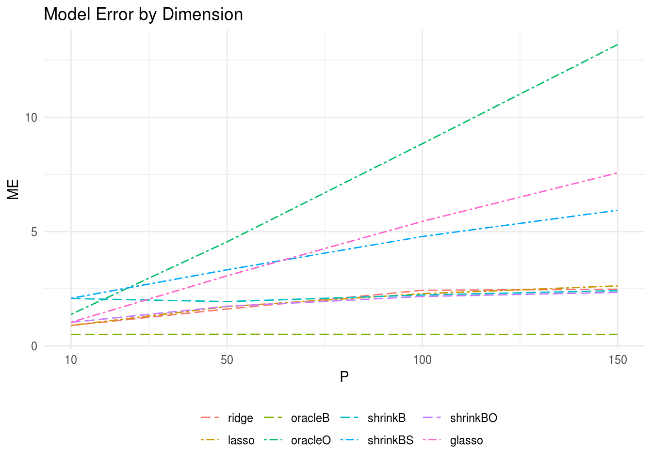
FIGURE 3.1: The oracle precision matrices were tri-diagonal with variable dimension (p) and the data was generated with sample size n = 100 and response vector dimension r = 10. The model errors (ME) for each estimator with variable dimension of the predictor matrix are plotted. shrinkBO and shrinkB were the two best-performing estimators closely follow by the ridge and lasso regression estimators.
| Model | Error | SD |
|---|---|---|
| oracleB | 0.5056 | 0.5122 |
| shrinkBO | 2.341 | 1.014 |
| shrinkB | 2.419 | 1.083 |
| ridge | 2.479 | 1.128 |
| lasso | 2.627 | 1.27 |
| shrinkBS | 5.932 | 4.001 |
| glasso | 7.57 | 5.412 |
| oracleO | 13.18 | 10.11 |
| OLS | 14.41 | 11.24 |
| oracleS | 52.07 | 44.62 |
3.3.1 Regression Simulations with Covariance Shrinkage
This final simulation was explored due to the fact that each of the SCPME regression estimators require an estimation of the cross-covariance matrix. In the previous simulations, we naively used the maximum likelihood estimate. However, because the data-generating procedure constructs settings that are inherently sparse, we were interested to determine if additional shrinkage of the maximum likelihood estimate for the cross-covariance matrix would also prove beneficial. For instance, in a number of settings, we were finding that the estimator oracleO was performing worse than oracleS. This perhaps suggests that estimating the covariance matrix \(\Sigma_{xy}\) well is more important than estimating \(\Omega\) well. This simulation explores that theory a bit further.
The data-generating procedure for this simulation is similar to previous one but here we take \(n = 100\), \(p = 200\), \(r = 10\), and, in addition, we multiply the population cross-covariance estimator by a factor of \(k\) where \(k \in (0.1, 0.2, ..., 0.9, 1)\). Figure 3.2 plots the MSPE for shrinkB for each tuning parameter, \(\lambda\), and constant, \(k\), pair. Figure 3.3 plots the MSPE similarly for shrinkBO.
Interestingly, we find that in this high dimension setting, it does appear that shrinking the sample covariance matrix by a constant factor helps the overall prediction performance of the SCPME estimators. This is indicated by the fact that the optimal constant, \(k\), hovers between 0.3 and 0.6 for each of the estimators. We also performed a simulation in low dimensions (not shown) but we did not see the same benefit.
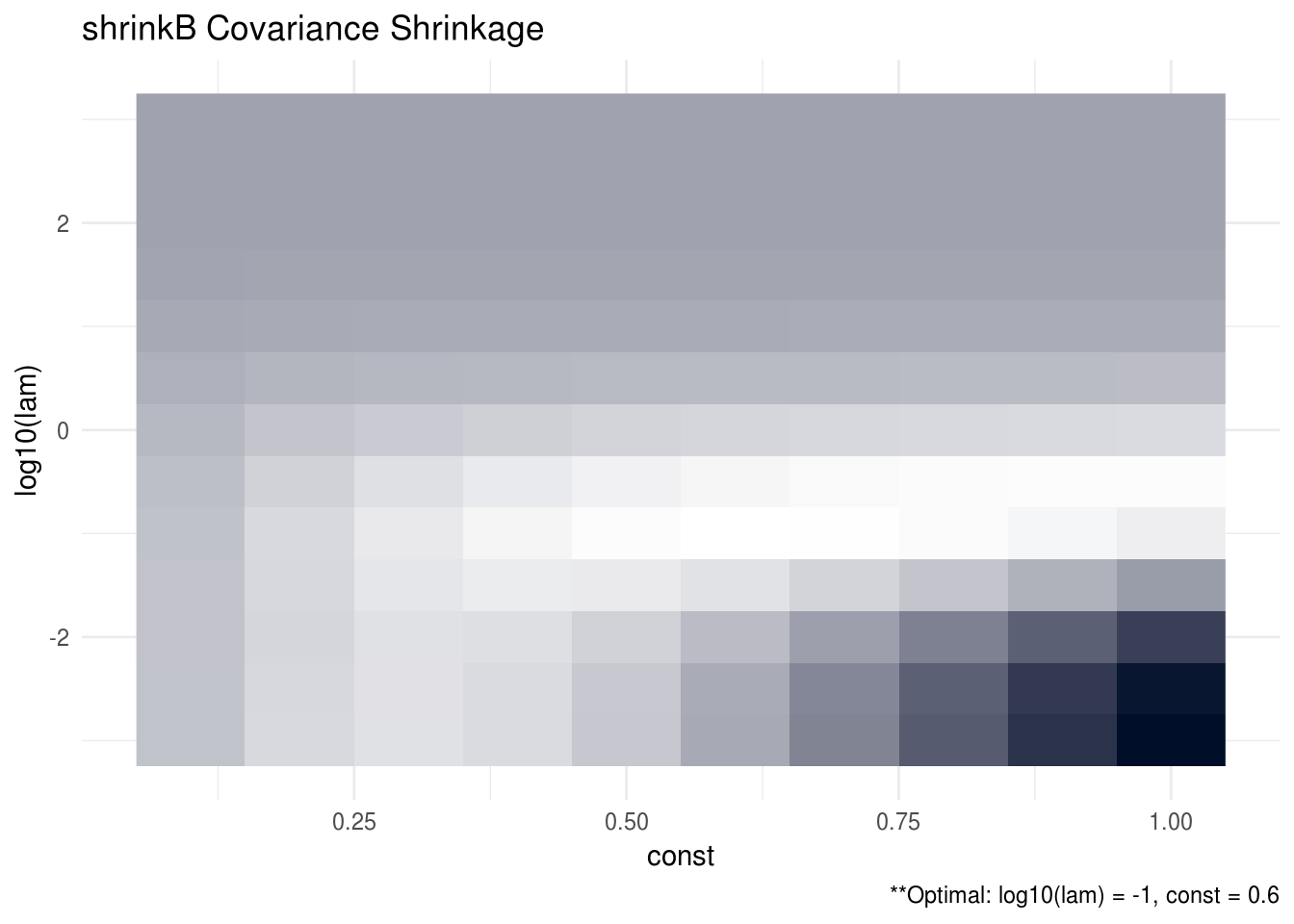
FIGURE 3.2: The oracle precision matrices were tri-diagonal with dimension p = 200 and the data was generated with a sample size n = 100 and response vector dimension r = 10. The cross validation MSPE are plotted for each lambda and constant tuning parameter pair. The optimal tuning parameter pair was found to be log10(lam) = -1 and const = 0.6. Note that brighter areas signify smaller losses.
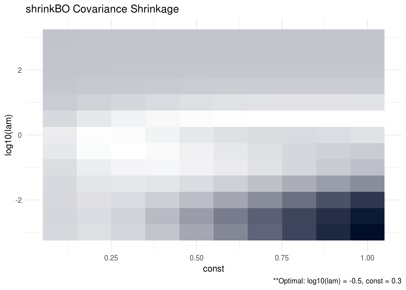
FIGURE 3.3: The oracle precision matrices were tri-diagonal with dimension p = 200 and the data was generated with a sample size n = 100 and response vector dimension r = 10. The cross validation MSPE are plotted for each lambda and constant tuning parameter pair. The optimal tuning parameter pair was found to be log10(lam) = -0.5 and const = 0.3. Note that brighter areas signify smaller losses.
3.4 Discussion
Apart from the two SCPME estimators discussed in the previous section, the generality of the SCPME framework allows for many previously unconceptualized precision matrix estimators to be explored. One estimator that was concieved of in our work but deserves further attention in future research is of the form
\[\begin{equation} \hat{\Omega}_{x} = \arg\min_{\Omega_{x} \in \mathbb{S}_{+}^{p}}\left\{ tr(S_{x}\Omega_{x}) - \log\left| \Omega_{x} \right| + \frac{\lambda}{2}\left\| \mathbb{X}\Omega_{x} \Sigma_{xy} - \mathbb{Y} \right\|_{F}^{2} \right\} \tag{3.18}\notag \end{equation}\]
For clarity in regards to the SCPME framework, \(A = \mathbb{X}, B = \Sigma_{xy}, \mbox{ and } C = \mathbb{Y}\). As before, \(\mathbb{X}\) is the \(n \times p\) matrix with rows \(X_{i} \in \mathbb{R}^{p}\) for \(i = 1,..., n\) and the script notation denotes that the matrix has been column-centered. The matrix \(\mathbb{Y}\) is a similar representation for the observed responses \(Y_{i} \in \mathbb{R}^{r}\). Also note that here we are using the Frobenius norm instead of the matrix \(l_{1}\)-norm but this replacement requires only a slight modification of the augmented ADMM algorithm for optimization - details of which will be presented later.
This optimization problem estimates a precision matrix that balances minimizing the gaussian negative log-likelihood for \(\Omega_{x}\) with minimizing the squared prediction error for the forward regression model. In other words, the objective function aims to penalize estimates, determined by \(\lambda\), that too heavily favor maximizing the marginal likelihood for \(X\) over the predictive performance of the conditional model \(Y\) given \(X\). This estimator also reveals an interesting connection to the joint log-likelihood of the two random variables. To see this, let us suppose that we have \(n\) independent copies of the random pair \((Y_{i}, X_{i})\) and we assume a linear relationship such that
\[\begin{equation} Y_{i} = \mu_{y} + \beta'\left(X_{i} - \mu_{x}\right) + E_{i} \end{equation}\]
where \(E_{i} \sim N_{r}\left( 0, \Omega_{y | x}^{-1} \right)\) and \(X_{i} \sim N_{p}\left( \mu_{x}, \Omega_{x}^{-1} \right)\). This implies that the conditional distribution of \(Y_{i}|X_{i}\) is of the form
\[\begin{equation} Y_{i} | X_{i} \sim N_{r}\left( \mu_{y} + \beta'\left(X_{i} - \mu_{x}\right), \Omega_{y | x}^{-1} \right) \end{equation}\]
We can use this conditional distribution along with the marginal distribution of \(X\) to derive the joint log-likelihood of \(X\) and \(Y\). Recall that \(\beta \equiv \Omega_{x}\Sigma_{xy}\) and \(S_{x}\) is the marginal sample covariance matrix of \(X\). Without loss of generality, we will assume here that \(\mu_{x} = \mu_{y} = 0\).
\[\begin{equation} \begin{split} l\left( \Omega_{y | x}, \Omega_{x}, \Sigma_{xy} | Y, X \right) &= constant + \frac{n}{2}\log\left| \Omega_{y | x} \right| - \frac{1}{2}\sum_{i = 1}^{n} tr\left[ \left( Y_{i} - \Sigma_{xy}'\Omega_{x} X_{i} \right)\left( Y_{i} - \Sigma_{xy}'\Omega_{x} X_{i} \right)'\Omega_{y | x} \right] \\ &+\frac{n}{2}\log\left| \Omega \right| - \frac{1}{2}\sum_{i = 1}^{n}tr\left( X_{i}X_{i}'\Omega_{x} \right) \\ &= constant + \frac{n}{2}\log\left| \Omega_{y | x} \right| - \frac{1}{2}tr\left[ \left( \mathbb{Y} - \mathbb{X}\Omega_{x}\Sigma_{xy} \right)'\left( \mathbb{Y} - \mathbb{X}\Omega_{x}\Sigma_{xy} \right)\Omega_{y | x} \right] \\ &+ \frac{n}{2}\log\left| \Omega_{x} \right| - \frac{n}{2}tr\left( S_{x}\Omega_{x} \right) \end{split} \tag{3.19}\notag \end{equation}\]
Optimizing this joint log-likelihood with respect to \(\Omega_{x}\) reveals strong similiarities to the estimator that was derived from the SCPME framework:
\[\begin{equation} \begin{split} \hat{\Omega}_{x} &= \arg\min_{\Omega_{x} \in \mathbb{S}_{+}^{p}}\left\{ \frac{1}{2}tr\left[ \left( \mathbb{Y} - \mathbb{X}\Omega_{x}\Sigma_{xy} \right)'\left( \mathbb{Y} - \mathbb{X}\Omega_{x}\Sigma_{xy} \right)\Omega_{y | x} \right] + \frac{n}{2}tr\left( S_{x}\Omega_{x} \right) - \frac{n}{2}\log\left| \Omega_{x} \right| \right\} \\ &= \arg\min_{\Omega_{x} \in \mathbb{S}_{+}^{p}}\left\{ tr\left( S_{x}\Omega_{x} \right) - \log\left| \Omega_{x} \right| + \frac{1}{n}\left\| \left( \mathbb{X}\Omega_{x}\Sigma_{xy} - \mathbb{Y} \right)\Omega_{y | x}^{1/2} \right\|_{F}^{2} \right\} \end{split} \tag{3.20}\notag \end{equation}\]
If it is the case that, given \(X\), each of the \(r\) responses are pairwise independent with equal variance so that \(\Omega_{y | x}^{1/2} = \sigma_{y | x}I_{r}\) and we let \(\lambda = 2\sigma_{y | x}^{2}/n\), then we have that
\[\begin{equation} \hat{\Omega}_{x} = \arg\min_{\Omega_{x} \in \mathbb{S}_{+}^{p}}\left\{ tr\left( S_{x}\Omega_{x} \right) - \log\left| \Omega_{x} \right| + \frac{\lambda}{2}\left\| \mathbb{X}\Omega_{x}\Sigma_{xy} - \mathbb{Y} \right\|_{F}^{2} \right\} \tag{3.21}\notag \end{equation}\]
This is exactly the estimator conceived of previously. Of course, throughout this derivation there were several assumptions that were made and in practice we do not know the true values of neither \(\Omega_{y | x}\) nor \(\Sigma_{xy}\). However, we can see that this estimator is solving a very similar problem to that of optimizing the joint log-likelihood with respect to \(\Omega_{x}\). We think this estimator and related ones deserve attention in future work.
The algorithm for solving this optimization problem is below. Note that no closed-form solution exists and so we must resort to some iterative algorithm similar to the SCPME augmented ADMM algorithm10. The only difference here is that in step four we no longer require elementwise soft-thresholding.
Theorem 3.2 (Modified Augmented ADMM Algorithm for Shrinking Characteristics of Precision Matrix Estimators with Frobenius Norm) Set \(k = 0\) and initialize \(Z^{0}, \Lambda^{0}, \Omega^{0}\), and \(\rho\) and repeat steps 1-5 until convergence.
Compute \(G^{k} = \rho A'\left( A\Omega^{k} B - Z^{k} - C + \rho^{-1}\Lambda^{k} \right)B'\)
Decompose \(S + \left( G^{k} + (G^{k})' \right)/2 - \rho\tau\Omega^{k} = VQV'\) (via the spectral decomposition).
Set \(\Omega^{k + 1} = V\left( -Q + (Q^{2} + 4\rho\tau I_{p})^{1/2} \right)V'/(2\rho\tau)\)
Set \(Z^{k + 1} = \left[ \rho\left( A\Omega^{k + 1} B - C \right) + \Lambda^{k} \right]/(\lambda + \rho)\)
- Set \(\Lambda^{k + 1} = \rho\left( A\Omega^{k + 1} B - Z^{k + 1} - C \right)\)
References
Cai, Tony, and Weidong Liu. 2011. “A Direct Estimation Approach to Sparse Linear Discriminant Analysis.” Journal of the American Statistical Association 106 (496). Taylor & Francis: 1566–77.
Dalal, Onkar, and Bala Rajaratnam. 2017. “Sparse Gaussian Graphical Model Estimation via Alternating Minimization.” Biometrika 104 (2). Oxford University Press: 379–95.
Fan, Jianqing, Yang Feng, and Xin Tong. 2012. “A Road to Classification in High Dimensional Space: The Regularized Optimal Affine Discriminant.” Journal of the Royal Statistical Society: Series B (Statistical Methodology) 74 (4). Wiley Online Library: 745–71.
Lange, Kenneth. 2016. MM Optimization Algorithms. Vol. 147. SIAM.
Mai, Qing, Hui Zou, and Ming Yuan. 2012. “A Direct Approach to Sparse Discriminant Analysis in Ultra-High Dimensions.” Biometrika 99 (1). Oxford University Press: 29–42.
Molstad, Aaron J, and Adam J Rothman. 2017. “Shrinking Characteristics of Precision Matrix Estimators.” Biometrika.
Witten, Daniela M, and Robert Tibshirani. 2009. “Covariance-Regularized Regression and Classification for High Dimensional Problems.” Journal of the Royal Statistical Society: Series B (Statistical Methodology) 71 (3). Wiley Online Library: 615–36.
Further explanation of the majorizing function (3.6) in section A.0.5↩
If \(Q\) is positive definite, then \(vec\left(\Omega - \Omega^{k} \right)'\rho Q\left(\Omega - \Omega^{k} \right)/2 > 0\) since \(\rho > 0\) and \(vec\left(\Omega - \Omega^{k}\right)\) is always nonzero whenever \(\Omega \neq \Omega^{k}\).↩