C SCPME R Package
SCPME is an R package that estimates a penalized precision matrix via a modified alternating direction method of multipliers (ADMM) algorithm as described in Molstad and Rothman (2017). Specifically, the modified ADMM algorithm solves the following optimization problem:
\[ \hat{\Omega} = \arg\min_{\Omega \in S_{+}^{p}}\left\{ tr\left(S \Omega\right) - \log\det\left(\Omega\right) + \lambda\left\| A\Omega B - C \right\|_{1} \right\} \]
where \(\lambda > 0\) is a tuning parameter, \(A, B, \mbox{ and } C\) are known, user-specified matrices, and we define \(\left\|A \right\|_{1} = \sum_{i, j} \left| A_{ij} \right|\).
This form of penalty leads to many new, interesting, and novel estimators for the precision matrix \(\Omega\). Users can construct matrices \(A, B, \mbox{ and } C\) so that emphasis is placed on the sum, absolute value of a characteristic of \(\Omega\). We will explore a few of these estimators in the tutorial section.
A list of functions contained in the package can be found below:
shrink()computes the estimated precision matrixdata_gen()data generation function (for convenience)plot.shrink()produces a heat map or optional line graph for the cross validation errors
C.1 Installation
# The easiest way to install is from CRAN
install.packages("SCPME")

# You can also install the development version from GitHub:
# install.packages('devtools')
devtools::install_github("MGallow/SCPME")
This package is hosted on Github at github.com/MGallow/SCPME. The project website is located at mattxgalloway.com/SCPME.
C.2 Tutorial
The primary function in the SCPME package is shrink(). The input values \(X\) is an \(n \times p\) data matrix so that there are \(n\) rows each representing an observation and \(p\) columns each representing a unique variable and \(Y\) is an \(n \times r\) response matrix where \(r\) is the dimension of the response vector. By default, SCPME will estimate \(\Omega\) using a lasso penalty (\(A = I_{p}, B = I_{p}, \mbox{ and } C = 0\)) and choose the optimal \(\lambda\) tuning parameter that minimizes the mean squared prediction error for the regression of the variable \(Y\) on \(X\) (here \(I_{p}\) denotes a \(p\)-dimension identity matrix). If \(Y\) is not provided, then tuning parameter selection will be based on the validation likelihood. Note that \(\Omega\) (perhaps better denoted here as \(\Omega_{x}\)) will only have meaningful shrinkage unless the data vector \(X \in \mathbb{R^{p}}\) is multi-dimensional (\(p > 1\)).
In this example, the data matrix is \(100 \times 5\) and the response is generated according to the following model:
\[ Y_{i} = \beta'X_{i} + E_{i} \]
where \(E_{i} \sim N\left( 0, 1 \right)\) and \(X_{i}\) is generated from a multivariate normal distribution with mean zero and tapered oracle covariance matrix \(S\). A tapered covariance matrix has the property that its inverse - the precision matrix - is tri-diagonal. Estimating this oracle precision matrix well and efficiently will be our primary interest. In addition, \(\beta\) is randomly generated and sparse. The data will be generated using the data_gen() function contained in the package.
library(SCPME)
set.seed(123)

# generate 100 x 5 X data matrix and 100 x 1 Y data matrix
data = data_gen(p = 5, n = 100, r = 1)

# the oracle regression coefficients are sparse
data$betas
## [,1]
## [1,] -0.25065233
## [2,] 0.00000000
## [3,] 0.69707555
## [4,] 0.03153231
## [5,] 0.00000000# shrink sum absolute entries in omega
shrink(X = data$X, Y = data$Y)##
## Call: shrink(X = data$X, Y = data$Y)
##
## Iterations: 37
##
## Tuning parameters:
## log10(lam) lam
## [1,] -1.163 0.069
##
## Log-likelihood: -178.20154
##
## Omega:
## [,1] [,2] [,3] [,4] [,5]
## [1,] 1.60847 -0.73553 -0.14094 -0.04329 -0.11730
## [2,] -0.73553 1.66045 -0.52579 -0.03576 -0.03342
## [3,] -0.14094 -0.52579 1.73410 -0.85121 -0.07332
## [4,] -0.04329 -0.03576 -0.85121 2.02541 -0.93612
## [5,] -0.11730 -0.03342 -0.07332 -0.93612 1.62397Notice here that the estimated precision matrix is not sparse. This is due to the fact that our cross validation criteria is the mean-squared prediction error. We can estimate a new precision matrix using the validation likelihood as the cross validation criteria with the following command:
# shrink sum absolute entries in omega
shrink(X = data$X, Y = data$Y, crit.cv = "loglik")
##
## Call: shrink(X = data$X, Y = data$Y, crit.cv = "loglik")
##
## Iterations: 51
##
## Tuning parameters:
## log10(lam) lam
## [1,] -2.163 0.007
##
## Log-likelihood: -120.02858
##
## Omega:
## [,1] [,2] [,3] [,4] [,5]
## [1,] 2.11926 -1.17294 -0.13784 -0.00678 -0.20014
## [2,] -1.17294 2.28420 -0.81629 0.00009 -0.00001
## [3,] -0.13784 -0.81629 2.45520 -1.42117 0.01650
## [4,] -0.00678 0.00009 -1.42117 3.09526 -1.56839
## [5,] -0.20014 -0.00001 0.01650 -1.56839 2.24703All of the estimators so far have used a lasso penalty that penalizes the sum of the absolute value of all the entries in \(\Omega\) (\(A = I_{p}, B = I_{p}, \mbox{ and } C = 0\)). In effect, this penalty embeds an assumption in our estimate that the true population precision matrix, \(\Omega\), is sparse. The flexibility of the penalty described in Molstad and Rothman (2017) allows us to make other assumptions as well. For instance, in the penalty we could set \(A = I_{p}, B = \Sigma_{xy}\) where \(\Sigma_{xy}\) is the covariance matrix of \(X\) and \(Y\), and \(C = 0\). In which case our penalty function
\[P_{\lambda}\left(\Omega \right) = \lambda\left\| A\Omega B - C \right\|_{1} = \lambda\left\| \Omega\Sigma_{xy} \right\|_{1} = \lambda\left\| \beta \right\|_{1} \]
This objective function estimates an \(\Omega\) via the marginal log-likelihood of \(X\) under the assumption that the forward regression coefficient \(\beta\) is sparse (recall that \(\beta \equiv \Omega\Sigma_{xy}\)). Of course, in practice, we do not know the true covariance matrix \(\Sigma_{xy}\) but we might consider using the sample estimate \(\hat{\Sigma}_{xy} = \sum_{i = 1}^{n}\left(X_{i} - \bar{X}\right)\left(Y_{i} - \bar{Y}\right)'/n\).
# assume sparsity in beta
lam_max = max(abs(crossprod(data$X, data$Y)))
(shrink = shrink(X = data$X, Y = data$Y, B = cov(data$X, data$Y),
    lam.max = lam_max, nlam = 20))
##
## Call: shrink(X = data$X, Y = data$Y, B = cov(data$X, data$Y), nlam = 20,
## lam.max = lam_max)
##
## Iterations: 84
##
## Tuning parameters:
## log10(lam) lam
## [1,] -0.167 0.681
##
## Log-likelihood: -133.98097
##
## Omega:
## [,1] [,2] [,3] [,4] [,5]
## [1,] 2.12467 -1.20016 -0.01149 0.01660 -0.20424
## [2,] -1.20016 2.28202 -0.70370 0.03047 -0.01211
## [3,] -0.01149 -0.70370 2.09284 -1.47505 0.01020
## [4,] 0.01660 0.03047 -1.47505 2.86829 -1.45784
## [5,] -0.20424 -0.01211 0.01020 -1.45784 2.18752Note that we specified the maximum lam value in the previous function to expand the tuning parameter grid. With these settings, the augmented ADMM algorithm also solves for the estimated \(\beta\) coefficient matrix simultaneously:
# print estimated beta matrix
shrink$Z
## [,1]
## [1,] 0.00000000
## [2,] 0.00000000
## [3,] 0.42221120
## [4,] 0.04782093
## [5,] 0.00000000Another possible penalty is to set \(B = \left[ \Sigma_{xy}, I_{p} \right]\) so that the identity matrix is appended to the covariance matrix of \(X\) and \(Y\). That is, the penalty \(P\), is constructed as
\[ P_{\lambda}\left(\Omega \right) = \lambda\left\| A\Omega B - C \right\|_{1} = \lambda\left\| \Omega\left[\Sigma_{xy}, I_{p}\right] \right\|_{1} = \lambda\left\| \beta \right\|_{1} + \lambda\left\| \Omega \right\|_{1} \]
In this case, we are equally penalizing the sum, absolute values of entries in \(\beta\) and \(\Omega\) which embeds an assumption that \(\beta\) and \(\Omega\) are both sparse.
# assume sparsity in beta AND omega
(shrink = shrink(X = data$X, Y = data$Y, B = cbind(cov(data$X,
    data$Y), diag(ncol(data$X))), lam.max = 10, lam.min.ratio = 1e-04,
    nlam = 20))
##
## Call: shrink(X = data$X, Y = data$Y, B = cbind(cov(data$X, data$Y),
## diag(ncol(data$X))), nlam = 20, lam.max = 10, lam.min.ratio = 1e-04)
##
## Iterations: 46
##
## Tuning parameters:
## log10(lam) lam
## [1,] 0.368 2.336
##
## Log-likelihood: -624.54758
##
## Omega:
## [,1] [,2] [,3] [,4] [,5]
## [1,] 0.26376 -0.00003 -0.00015 -0.00010 -0.00005
## [2,] -0.00003 0.24002 -0.00017 -0.00012 -0.00006
## [3,] -0.00015 -0.00017 0.19066 -0.00516 -0.00020
## [4,] -0.00010 -0.00012 -0.00516 0.20362 -0.00014
## [5,] -0.00005 -0.00006 -0.00020 -0.00014 0.22750# print estimated beta
shrink$Z[, 1, drop = FALSE]## [,1]
## [1,] 0.06389361
## [2,] 0.08542992
## [3,] 0.14200713
## [4,] 0.12357129
## [5,] 0.09958374SCPME also has the capability to provide plots (heatmaps and line graphs) for the cross validation errors. In the heatmap plot below, the more bright, white areas correspond to a better tuning parameter selection (lower cross validation error).
# produce CV heat map
plot(shrink, type = "heatmap")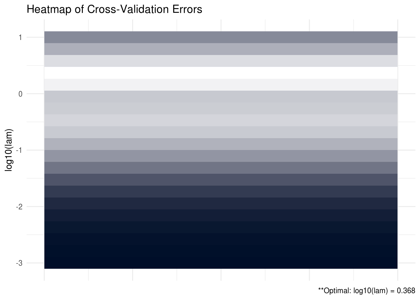
FIGURE C.1: CV heatmap for SCPME tutorial
# produce line graph
plot(shrink, type = "line")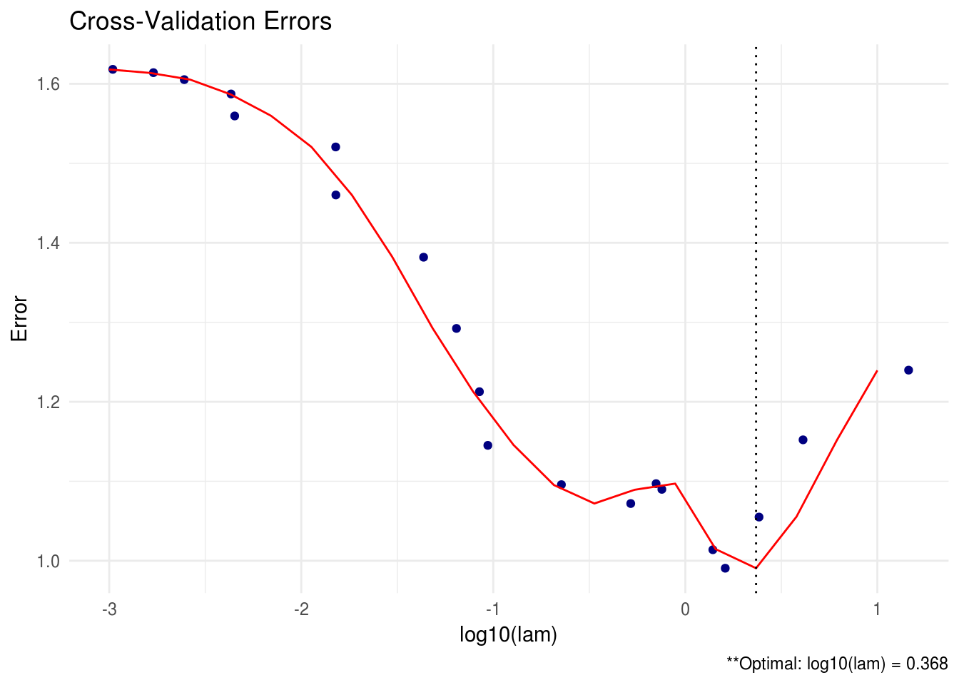
FIGURE C.2: CV line graph for SCPME tutorial
SCPME has a number of more advanced options including alternative convergence criteria and parallel CV that are explained in detail on the project website at mattxgalloway.com/SCPME.
References
Molstad, Aaron J, and Adam J Rothman. 2017. “Shrinking Characteristics of Precision Matrix Estimators.” Biometrika.