B ADMMsigma R Package
ADMMsigma is an R package that estimates a penalized precision matrix, often denoted \(\Omega\), via the alternating direction method of multipliers (ADMM) algorithm. Though not the fastest estimation method, the ADMM algorithm is easily adaptable and allows for rapid experimentation by the user, which is the primary goal of this package.
The package currently supports a general elastic-net penalty that allows for both ridge and lasso-type penalties as special cases. In particular, the algorithm solves the following optimization problem:
\[ \hat{\Omega} = \arg\min_{\Omega \in S_{+}^{p}}\left\{tr(S\Omega) - \log\det\left(\Omega\right) + \lambda\left[\frac{1 - \alpha}{2}\left\|\Omega\right\|_{F}^{2} + \alpha\left\|\Omega\right\|_{1} \right] \right\} \]
where \(\lambda > 0\), \(0 \leq \alpha \leq 1\) are tuning parameters, \(\left\|\cdot \right\|_{F}^{2}\) is the Frobenius norm, and we define \(\left\|A \right\|_{1} = \sum_{i, j} \left| A_{ij} \right|\).
A list of functions contained in the package can be found below:
ADMMsigma()computes the estimated precision matrix via the ADMM algorithm (ridge, lasso, and elastic-net regularization optional)RIDGEsigma()computes the estimated ridge penalized precision matrix via closed-form solutionplot.ADMMsigma()produces a heat map or optional line graph for cross validation errorsplot.RIDGEsigma()produces a heat map or optional line graph for cross validation errors
B.1 Installation
# The easiest way to install is from CRAN
install.packages("ADMMsigma")

# You can also install the development version from GitHub:
# install.packages('devtools')
devtools::install_github("MGallow/ADMMsigma")
This package is hosted on Github at github.com/MGallow/ADMMsigma. The project website is located at mattxgalloway.com/ADMMsigma.
B.2 Tutorial
By default, ADMMsigma will estimate a penalized precision matrix, \(\Omega\), using the elastic-net penalty and choose the optimal \(\lambda\) and \(\alpha\) tuning parameters. The primary function is simply ADMMsigma(). The input value \(X\) is an \(n \times p\) data matrix so that there are \(n\) rows each representing an observation and \(p\) columns each representing a unique feauture or variable.
Here, we will use a \(100 \times 5\) data matrix that is generated from a multivariate normal distribution with mean zero and tapered oracle covariance matrix \(S\). A tapered covariance matrix has an inverse - or precision matrix - that is tri-diagonal, which is useful for illustration purposes because the object is sparse (many zero entries) and the shrinkage penalty should prove useful.
# elastic-net type penalty (set tolerance to 1e-8)
ADMMsigma(X, tol.abs = 1e-08, tol.rel = 1e-08)
##
## Call: ADMMsigma(X = X, tol.abs = 1e-08, tol.rel = 1e-08)
##
## Iterations: 48
##
## Tuning parameters:
## log10(lam) alpha
## [1,] -1.599 1
##
## Log-likelihood: -108.41003
##
## Omega:
## [,1] [,2] [,3] [,4] [,5]
## [1,] 2.15283 -1.26902 0.00000 0.00000 0.19765
## [2,] -1.26902 2.79032 -1.32206 -0.08056 0.00925
## [3,] 0.00000 -1.32206 2.85470 -1.17072 -0.00865
## [4,] 0.00000 -0.08056 -1.17072 2.49554 -1.18959
## [5,] 0.19765 0.00925 -0.00865 -1.18959 1.88121We can see that the optimal \(\alpha\) value selected is one. This selection corresponds with a lasso penalty – a special case of the elastic-net penalty.
We can also explicitly assume sparsity in our estimate rather than let the package decide by restricting the class of penalties to the lasso. We do this by simply setting alpha = 1 in our function:
# lasso penalty (default tolerance)
ADMMsigma(X, alpha = 1)
##
## Call: ADMMsigma(X = X, alpha = 1)
##
## Iterations: 24
##
## Tuning parameters:
## log10(lam) alpha
## [1,] -1.599 1
##
## Log-likelihood: -108.41193
##
## Omega:
## [,1] [,2] [,3] [,4] [,5]
## [1,] 2.15308 -1.26962 0.00000 0.00000 0.19733
## [2,] -1.26962 2.79103 -1.32199 -0.08135 0.00978
## [3,] 0.00000 -1.32199 2.85361 -1.16953 -0.00921
## [4,] 0.00000 -0.08135 -1.16953 2.49459 -1.18914
## [5,] 0.19733 0.00978 -0.00921 -1.18914 1.88096ADMMsigma also has the capability to provide plots for the cross validation errors. This allows the user to analyze and manually select the appropriate tuning parameters. In the heatmap plot below, the bright, white areas of the heat map correspond to a better tuning parameter selection (low validation error). In the line graph, each line corresponds to a different \(\alpha\) tuning parameter.
# produce CV heat map for ADMMsigma
ADMM = ADMMsigma(X, tol.abs = 1e-08, tol.rel = 1e-08)
plot(ADMM, type = "heatmap")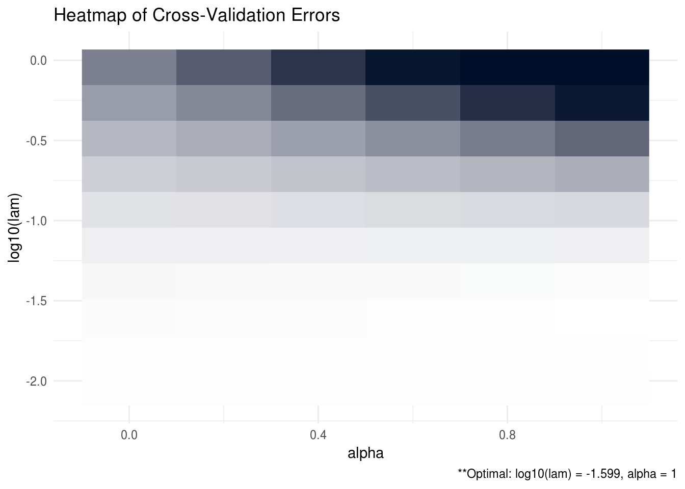
FIGURE B.1: CV heatmap for ADMMsigma tutorial.
# produce line graph for CV errors for ADMMsigma
plot(ADMM, type = "line")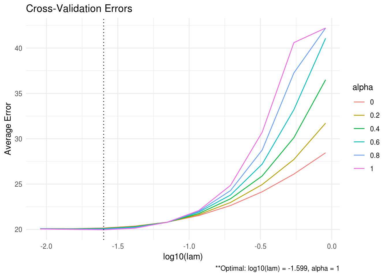
FIGURE B.2: CV line graph for ADMMsigma tutorial.
ADMMsigma has a number of more advanced options such as cross validation criteria, regularization path, and parallel CV that are explained in more detail on the project website at mattxgalloway.com/ADMMsigma.