Chapter 2 Precision Matrix Estimation
2.1 Background
The foundation of much of the precision matrix estimation literature is the gaussian negative log-likelihood. Consider the case where we observe \(n\) independent, identically distributed (iid) copies of the random variable \(X\), where the \(i\)th observation \(X_{i} \in \mathbb{R}^{p}\) is normally distributed with mean, \(\mu\), and variance, \(\Omega^{-1}\). That is, \(X_{i}\) follows a \(p\)-dimensional normal distribution which is typically denoted as \(X_{i} \sim N_{p}\left( \mu, \Omega^{-1} \right)\). By definition, this multivariate formulation implies the probability distribution function, \(f\), is of the form
\[\begin{equation} f\left(X_{i}; \mu, \Omega\right) = (2\pi)^{-p/2}\left| \Omega \right|^{1/2}\exp\left[ -\frac{1}{2}\left( X_{i} - \mu \right)'\Omega\left( X_{i} - \mu \right) \right] \tag{2.1}\notag \end{equation}\]
Furthermore, because we assume that each observation is independent, the probability distribution function for all \(n\) observations \(X_{1}, ..., X_{n}\) is equal to
\[\begin{equation} \begin{split} f\left(X_{1}, ..., X_{n}; \mu, \Omega\right) &= \prod_{i = 1}^{n}(2\pi)^{-p/2}\left| \Omega \right|^{1/2}\exp\left[ -\frac{1}{2}\left( X_{i} - \mu \right)'\Omega\left( X_{i} - \mu \right) \right] \\ &= (2\pi)^{-np/2}\left| \Omega \right|^{n/2}\mbox{etr}\left[ -\frac{1}{2}\sum_{i = 1}^{n}\left( X_{i} - \mu \right)\left( X_{i} - \mu \right)'\Omega \right] \end{split} \tag{2.2}\notag \end{equation}\]
Therefore, the gaussian log-likelihood, \(l\), for \(\mu\) and \(\Omega\) given \(X = (X_{1}, .., X_{n})\) can be written as
\[\begin{equation} l(\mu, \Omega | X) = constant + \frac{n}{2}\log\left| \Omega \right| - tr\left[ \frac{1}{2}\sum_{i = 1}^{n}\left(X_{i} - \mu \right)\left(X_{i} - \mu \right)'\Omega \right] \tag{2.3}\notag \end{equation}\]
The estimator for \(\mu\) that maximizes the log-likelihood is \(\hat{\mu}^{mle} = \bar{X} \equiv \sum_{i = 1}^{n}X_{i}/n\), so that the partially maximized gaussian log-likelihood function for \(\Omega\) is
\[\begin{equation} \begin{split} l(\Omega | X) &= \frac{n}{2}\log\left| \Omega \right| - tr\left[ \frac{1}{2}\sum_{i = 1}^{n}\left(X_{i} - \bar{X} \right)\left(X_{i} - \bar{X} \right)'\Omega \right] \\ &= \frac{n}{2}\log\left| \Omega \right| - \frac{n}{2}tr\left( S\Omega \right) \end{split} \tag{2.4}\notag \end{equation}\]
where \(S = \sum_{i = 1}^{n}\left(X_{i} - \bar{X}\right)\left(X_{i} - \bar{X}\right)'/n\) is the usual sample estimator for the population covariance matrix, \(\Sigma\). In addition to \(\mu\), one could also derive the maximum likelihood estimator for \(\Omega\). By setting the gradient of the partially maximized log-likelihood equal to zero, one could show that
\[\begin{equation} \begin{split} \hat{\Omega}^{mle} &= \arg\max_{\Omega \in S_{+}^{p}}\left\{ \frac{n}{2}\log\left| \Omega \right| - \frac{n}{2}tr\left(S\Omega \right) \right\} \\ &= \arg\min_{\Omega \in S_{+}^{p}}\left\{ tr\left(S\Omega\right) - \log\left|\Omega\right| \right\} \\ &= S^{-1} \end{split} \tag{2.5}\notag \end{equation}\]
so that the MLE for \(\Omega\), when it exists, is \(\hat{\Omega}^{mle} = S^{-1} = \left[\sum_{i = 1}^{n}\left(X_{i} - \bar{X}\right)\left(X_{i} - \bar{X}\right)'/n \right]^{-1}\). The reality, however, is that this object does not always exist. In settings where the number of observations is exceeded by the number of features in a sample, the sample covariance matrix is rank deficient and no longer invertible. For this reason, many papers in the last decade have proposed shrinkage estimators of the population precision matrix similar to the shrinkage estimators in regression settings. That is, instead of minimizing solely the negative log-likelihood function, researchers have proposed minimizing the gaussian log-likelihood plus a penalty term, \(P\), where \(P\) is often a function of the precision matrix.
\[\begin{equation} \hat{\Omega} = \arg\min_{\Omega \in S_{+}^{p}}\left\{ tr\left(S\Omega\right) - \log\left|\Omega \right| + P\left( \Omega \right) \right\} \tag{2.6} \end{equation}\]
The penalties that have been proposed for precision matrix estimation are typically a variation of the ridge penalty \(P\left(\Omega \right) = \lambda\|\Omega \|_{F}^{2}/2\) or the lasso penalty \(P\left(\Omega \right) = \lambda\left\|\Omega\right\|_{1}\) (here \(\lambda\) is a tuning parameter). The authors, Yuan and Lin (2007), initially proposed the lasso-penalized gaussian log-likelihood defined as
\[\begin{equation} \hat{\Omega} = \arg\min_{\Omega \in S_{+}^{p}}\left\{ tr\left(S\Omega\right) - \log\left|\Omega \right| + \lambda\sum_{i \neq j}\left|\Omega_{ij}\right| \right\} \tag{2.7} \end{equation}\]
so as not to penalize the diagonal elements of the precision matrix estimate. Other papers published on the lasso-penalized gaussian likelihood precision matrix estimator include Rothman et al. (2008) and Friedman, Hastie, and Tibshirani (2008). In addition, many efficient algorithms have been proposed to solve for \(\hat{\Omega}\), however, the most popular method is the graphical lasso algorithm (glasso) introduced by Friedman, Hastie, and Tibshirani (2008). Their method utilizes an iterative block-wise coordinate descent algorithm that builds upon the coordinate descent algorithm used in lasso-penalized regression.
Non-lasso, non-convex penalties were considered in Lam and Fan (2009) and Fan, Feng, and Wu (2009) and other papers considered penalizations like the Frobenius norm (Rothman, Forzani, and others (2014); Witten and Tibshirani (2009); Price, Geyer, and Rothman (2015)). In fact, the latter two papers show that the resulting minimizer can be solved in closed-form - which will be discussed later in this manuscript. However, the penalty explored through the remainder of this chapter is not a lasso penality nor a ridge penalty but, in fact, a convex combination of the two known as the elastic-net penalty:
\[\begin{equation} P\left( \Omega \right) = \lambda\left[\frac{1 - \alpha}{2}\left\| \Omega \right\|_{F}^{2} + \alpha\left\| \Omega \right\|_{1} \right] \tag{2.8}\notag \end{equation}\]
with additional tuning parameter \(0 \leq \alpha \leq 1\). Clearly, when \(\alpha = 0\) this penalty reduces to a ridge penalty and when \(\alpha = 1\) it reduces to a lasso penalty. Originally proposed in Zou and Hastie (2005) in the context of regression, this penalty has since been popularized and is used in the penalized regression R package glmnet. This penalty allows for additional flexibility but, despite this, no published work to our knowledge has explored the elastic-net penalty in the context of precision matrix estimation. We will show how to solve the following optimization problem in the next section using the ADMM algorithm.
\[\begin{equation} \hat{\Omega} = \arg\min_{\Omega \in S_{+}^{p}}\left\{ tr\left(S\Omega\right) - \log\left|\Omega \right| + \lambda\left[\frac{1 - \alpha}{2}\left\| \Omega \right|_{F}^{2} + \alpha\left\| \Omega \right\|_{1} \right] \right\} \tag{2.9} \end{equation}\]
2.2 ADMM Algorithm
ADMM stands for alternating direction method of multipliers. The algorithm was largely popularized by Stephen Boyd and his fellow authors in the book Distributed Optimization and Statistical Learning via the Alternating Direction Method of Multipliers (Boyd et al. 2011). As the authors state in the text, the “ADMM is an algorithm that is intended to blend the decomposability of dual ascent with the superior convergence properties of the method of multipliers.” By closely following Boyd’s descriptions and guidance in the published text, we will show in this section that the ADMM algorithm is particularly well-suited to solve the penalized log-likelihood optimization problem we are interested in here.
In general, the ADMM algorithm supposes that we want to solve an optimization problem of the form
\[\begin{equation} \begin{split} \mbox{minimize } f(x) + g(z) \\ \mbox{subject to } Ax + Bz = c \end{split} \tag{2.10}\notag \end{equation}\]
where we can assume here that \(x \in \mathbb{R}^{n}, z \in \mathbb{R}^{m}, A \in \mathbb{R}^{p \times n}, B \in \mathbb{R}^{p \times m}\), \(c \in \mathbb{R}^{p}\), and \(f\) and \(g\) are convex functions. In order to find the pair \((x^{*}, z^{*})\) that achieves the infimum, the ADMM algorithm uses an augmented lagrangian, \(L\), which Boyd et al. (2011) define as
\[\begin{equation} L_{\rho}(x, z, y) = f(x) + g(z) + y'(Ax + Bz - c) + \frac{\rho}{2}\left\| Ax + Bz - c \right\|_{2}^{2} \tag{2.11}\notag \end{equation}\]
In this formulation, \(y \in \mathbb{R}^{p}\) is called the lagrange multiplier and \(\rho > 0\) is some scalar that acts as the step size for the algorithm. Note that any infimum under the augmented lagrangian is equivalent to the infimum of the traditional lagrangian since any feasible point \((x, z)\) must satisfy the constraint \(\rho\left\| Ax + Bz - c \right\|_{2}^{2}/2 = 0\). Boyd et al. (2011) show that using the ADMM algorithm the infimum will be approached under the following repeated iterations:
\[\begin{equation} \begin{split} x^{k + 1} &= \arg\min_{x \in \mathbb{R}^{n}}L_{\rho}(x, z^{k}, y^{k}) \\ z^{k + 1} &= \arg\min_{z \in \mathbb{R}^{m}}L_{\rho}(x^{k + 1}, z, y^{k}) \\ y^{k + 1} &= y^{k} + \rho(Ax^{k + 1} + Bz^{k + 1} - c) \end{split} \tag{2.12}\notag \end{equation}\]
where the superscript, \(k\), denotes the number of iterations. Conveniently, this general algorithm can be coerced into a format useful in precision matrix estimation. Suppose we let \(f\) be equal to the non-penalized gaussian log-likelihood, \(g\) equal to the elastic-net penalty, \(P\left( \Omega \right)\), and we use the constraint that \(\Omega \in \mathbb{S}_{+}^{p}\) must be equal to some matrix \(Z \in \mathbb{R}^{p \times p}\), then the augmented lagrangian in the context of precision matrix estimation is of the form
\[\begin{equation} L_{\rho}(\Omega, Z, \Lambda) = f\left(\Omega\right) + g\left(Z\right) + tr\left[\Lambda\left(\Omega - Z\right)\right] + \frac{\rho}{2}\left\|\Omega - Z\right\|_{F}^{2} \tag{2.13}\notag \end{equation}\]
where \(\Lambda\) takes the role of \(y\) as the lagrange multiplier. The ADMM algorithm now consists of the following repeated iterations:
\[\begin{equation} \begin{split} \Omega^{k + 1} &= \arg\min_{\Omega \in \mathbb{S}_{+}^{p}}\left\{ tr\left(S\Omega\right) - \log\left|\Omega\right| + tr\left[\Lambda^{k}\left(\Omega - Z^{k}\right)\right] + \frac{\rho}{2}\left\| \Omega - Z^{k} \right\|_{F}^{2} \right\} \\ Z^{k + 1} &= \arg\min_{Z \in \mathbb{S}^{p}}\left\{ \lambda\left[ \frac{1 - \alpha}{2}\left\| Z \right\|_{F}^{2} + \alpha\left\| Z \right\|_{1} \right] + tr\left[\Lambda^{k}\left(\Omega^{k + 1} - Z\right)\right] + \frac{\rho}{2}\left\| \Omega^{k + 1} - Z \right\|_{F}^{2} \right\} \\ \Lambda^{k + 1} &= \Lambda^{k} + \rho\left( \Omega^{k + 1} - Z^{k + 1} \right) \end{split} \tag{2.14} \end{equation}\]
Furthermore, it turns out that each step in this algorithm can be solved efficiently in closed-form. The full details of each can be found in the appendix A.0.1 but the following theorem provides the simplified steps in the algorithm.
Theorem 2.1 (ADMM Algorithm for Elastic-Net Penalized Precision Matrix Estimation) Define the soft-thresholding function as \(\mbox{soft}(a, b) = \mbox{sign}(a)(\left| a \right| - b)_{+}\) and \(S\) as the sample covariance matrix. Set \(k = 0\) and initialize \(Z^{0}, \Lambda^{0}\), and \(\rho\). Repeat steps 1-3 until convergence:
- Decompose \(S + \Lambda^{k} - \rho Z^{k} = VQV'\) via spectral decomposition1. Then
\[\begin{equation} \Omega^{k + 1} = \frac{1}{2\rho}V\left[ -Q + \left( Q^{2} + 4\rho I_{p} \right)^{1/2} \right]V' \tag{2.15} \end{equation}\]
- Elementwise soft-thresholding for all \(i = 1,..., p\) and \(j = 1,..., p\)2.
\[\begin{equation} \begin{split} Z_{ij}^{k + 1} &= \frac{1}{\lambda(1 - \alpha) + \rho}\mbox{sign}\left(\rho\Omega_{ij}^{k + 1} + \Lambda_{ij}^{k}\right)\left( \left| \rho\Omega_{ij}^{k + 1} + \Lambda_{ij}^{k} \right| - \lambda\alpha \right)_{+} \\ &= \frac{1}{\lambda(1 - \alpha) + \rho}\mbox{soft}\left(\rho\Omega_{ij}^{k + 1} + \Lambda_{ij}^{k}, \lambda\alpha\right) \end{split} \tag{2.16} \end{equation}\]
- Update \(\Lambda^{k + 1}\).
\[\begin{equation} \Lambda^{k + 1} = \Lambda^{k} + \rho\left( \Omega^{k + 1} - Z^{k + 1} \right) \tag{2.17}\notag \end{equation}\]
2.2.1 Scaled-Form ADMM
Another popular, alternative form of the ADMM algorithm can be used when scaling the dual variable (\(\Lambda^{k}\)) which we will briefly mention in the context of precision matrix estimation here.
Define \(R^{k} = \Omega - Z^{k}\) and \(U^{k} = \Lambda^{k}/\rho\) then
\[\begin{equation} \begin{split} tr\left[ \Lambda^{k}\left( \Omega - Z^{k} \right) \right] + \frac{\rho}{2}\left\| \Omega - Z^{k} \right\|_{F}^{2} &= tr\left[ \Lambda^{k}R^{k} \right] + \frac{\rho}{2}\left\| R^{k} \right\|_{F}^{2} \\ &= \frac{\rho}{2}\left\| R^{k} + \Lambda^{k}/\rho \right\|_{F}^{2} - \frac{\rho}{2}\left\| \Lambda^{k}/\rho \right\|_{F}^{2} \\ &= \frac{\rho}{2}\left\| R^{k} + U^{k} \right\|_{F}^{2} - \frac{\rho}{2}\left\| U^{k} \right\|_{F}^{2} \end{split} \tag{2.18}\notag \end{equation}\]
Therefore, a scaled-form ADMM algorithm can now be written as
\[\begin{equation} \begin{split} \Omega^{k + 1} &= \arg\min_{\Omega \in \mathbb{S}_{+}^{p}}\left\{ tr\left(S\Omega\right) - \log\left|\Omega\right| + \frac{\rho}{2}\left\| \Omega - Z^{k} + U^{k} \right\|_{F}^{2} \right\} \\ Z^{k + 1} &= \arg\min_{Z \in \mathbb{S}^{p}}\left\{ \lambda\left[ \frac{1 - \alpha}{2}\left\| Z \right\|_{F}^{2} + \alpha\left\| Z \right\|_{1} \right] + \frac{\rho}{2}\left\| \Omega^{k + 1} - Z + U^{k} \right\|_{F}^{2} \right\} \\ U^{k + 1} &= U^{k} + \Omega^{k + 1} - Z^{k + 1} \end{split} \tag{2.19} \end{equation}\]
Note that there are limitations to using this method. Because the dual variable is scaled by \(\rho\) (the step size), this form limits one to using a constant step size for all \(k\) steps if no further adjustments are made to \(U^{k}\).
2.2.2 Stopping Criterion
There are three optimality conditions for the ADMM algorithm that we can use to inform the convergence and stopping criterion. These general conditions were outlined in Boyd et al. (2011) but here we cater them to precision matrix estimation. The first condition is the primal optimality condition \(\Omega^{k + 1} - Z^{k + 1} = 0\) and the other two conditions are the dual conditions \(0 \in \partial f\left(\Omega^{k + 1}\right) + \Lambda^{k + 1}\) and \(0 \in \partial g\left(Z^{k + 1}\right) - \Lambda^{k + 1}\). The first dual optimality condition is a result of taking the sub-differential of the lagrangian (non-augmented) with respect to \(\Omega^{k + 1}\) and the second is a result of taking the sub-differential of the lagrangian with respect to \(Z^{k + 1}\). Note that in the first condition we must honor the symmetric constraint in \(\Omega\) but the second condition does not require it.
If we define the left-hand side of the primal optimality condition as the primal residual \(r^{k + 1} = \Omega^{k + 1} - Z^{k + 1}\), then at convergence we must require that \(r^{k + 1} \approx 0\). Likewise, if we define the dual residual \(s^{k + 1} = \rho\left( Z^{k + 1} - Z^{k} \right)\), we must also require that \(s^{k + 1} \approx 0\) for proper convergence. This dual residual is the direct result of the fact that \(\Omega^{k + 1}\) is the minimizer of the augmented lagragian3 so that \(0 \in \partial L_{p}\left( \Omega, Z^{k}, \Lambda^{k} \right)\) and consequently \(0 \in \rho\left( Z^{k + 1} - Z^{k} \right)\)4.
Combining these three optimality conditions, Boyd suggests a stopping criterion similar to \(\epsilon^{pri} \leq \left\| r^{k + 1} \right\|_{F}\) and \(\epsilon^{dual} \leq \left\| s^{k + 1} \right\|_{F}\) where \(\epsilon^{rel} = \epsilon^{abs} = 10^{-3}\) and \[\begin{equation} \begin{split} \epsilon^{pri} &= p\epsilon^{abs} + \epsilon^{rel}\max\left\{ \left\| \Omega^{k + 1} \right\|_{F}, \left\| Z^{k + 1} \right\|_{F} \right\} \\ \epsilon^{dual} &= p\epsilon^{abs} + \epsilon^{rel}\left\| \Lambda^{k + 1} \right\|_{F} \end{split} \tag{2.20}\notag \end{equation}\]
2.3 Simulations
As a proof-of-concept that the elastic-net penalty in the context of precision matrix estimation can provide useful results and that the ADMM algorithm used in this process works, this section offers a short simulation. For the simulation, we generated data from multiple, unique precision matrices with various oracle structures. For each data-generating procedure, the algorithm was run with a 5-fold cross validation to tune parameters \(\lambda\) and \(\alpha\). After 20 replications, the cross validation errors were totalled and the optimal tuning parameters were selected (results are in the top half of the figures). These results were then compared with the Kullback Leibler (KL) losses between the estimated matrices and the oracle matrices (results are in the bottom half of the figures).
The first figure shows the results when the data was generated from a multivariate normal distribution with mean equal to zero and a tri-diagonal oracle precision matrix. This oracle matrix was first generated as \(\left(S_{ij}\right) = 0.7^{\left|i - j \right|}\) for \(i,j = 1,..., p\) and then inverted. The results show that because the oracle precision matrix is sparse, the algorithm correctly chooses a sparse solution with \(\alpha = 1\) - indicating a lasso penalty.
The second figure shows the results when the data was generated from a multivariate normal distribution with mean equal to zero and a dense oracle precision matrix (non-sparse). Here, we randomly generated an orthogonal basis, set all eigen values equal to 1000, and then combined the matrices using QR decomposition. Interestingly, we find that the optimal \(\alpha\) in this case is 0.6 which closely matches the optimal result based on the KL loss. This shows that there are cases where an elastic-net penalty can provide useful results and that using only a lasso penalty may unnecessarily restrict our penalized estimation.
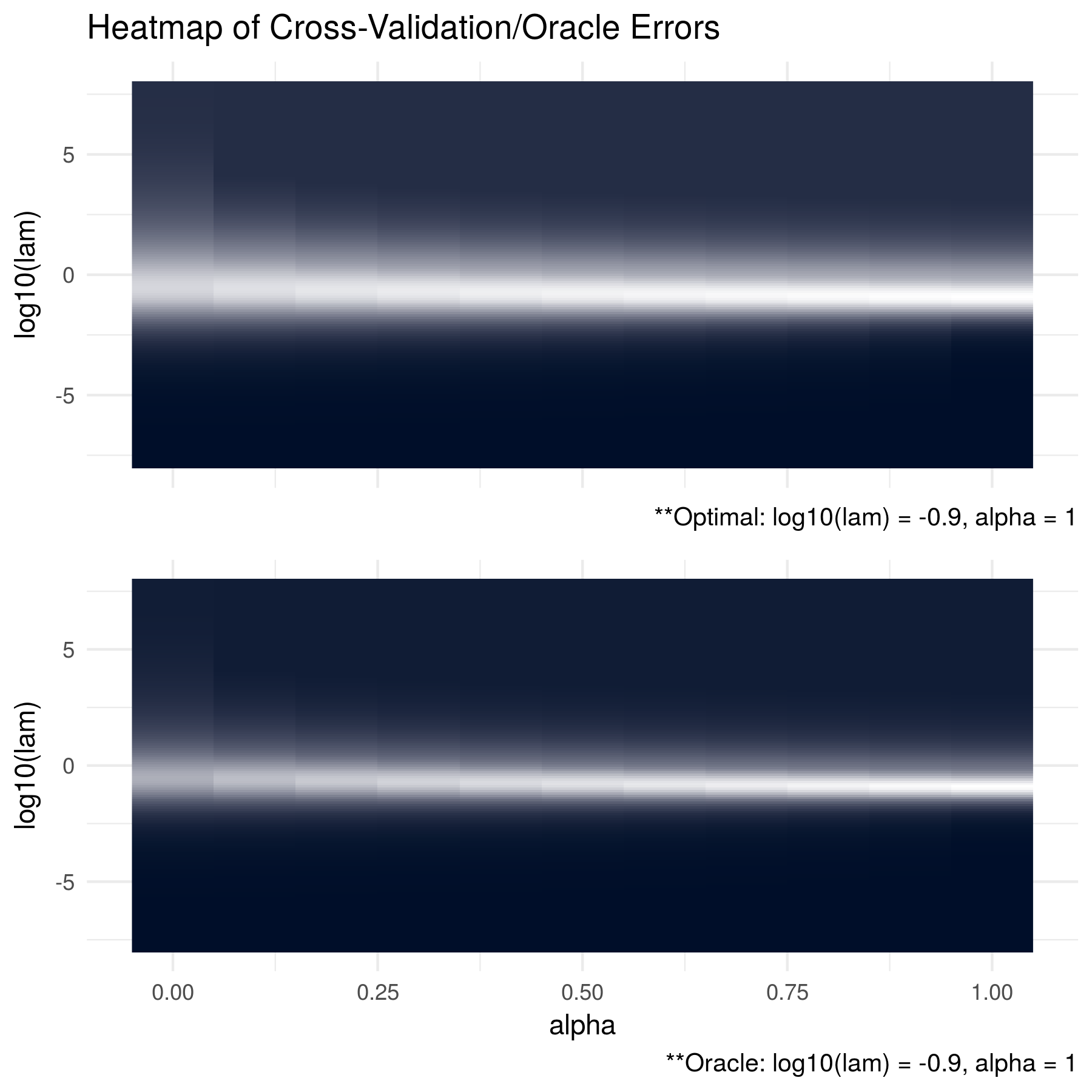
FIGURE 2.1: The oracle precision matrices were tri-diagonal with dimension p = 100 and the data was generated with a sample size of n = 50. The cross validation errors are in the top figure and the KL losses between the estimated matrices and the oracle matrices are shown in the bottom figure. The optimal tuning parameter pair for each heatmap was found to be log10(lam) = -0.9 and alpha = 1. Note that brighter areas signify smaller losses.
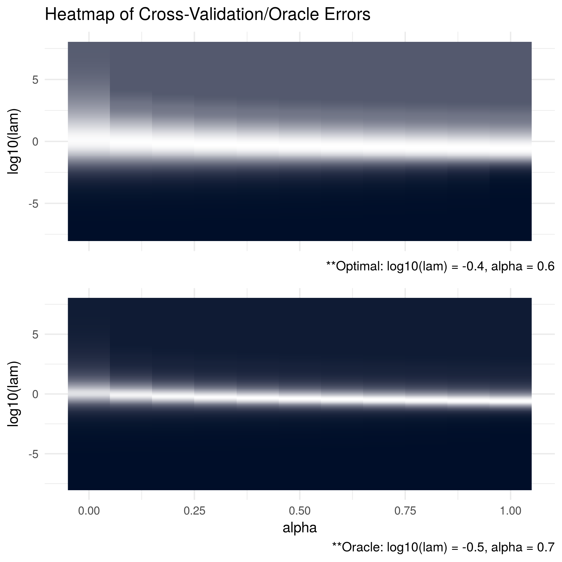
FIGURE 2.2: The oracle precision matrices were dense with dimension p = 100 and the data was generated with a sample size of n = 50. The cross validation errors are in the top figure and the KL losses between the estimated matrices and the oracle matrices are shown in the bottom figure. The optimal tuning parameter pair for the cross validation errors was found to be log10(lam) = -0.4 and alpha = 0.6 and log10(lam) = -0.5 and alpha = 0.7 for the KL losses. Note that brighter areas signify smaller losses.
References
Boyd, Stephen, Neal Parikh, Eric Chu, Borja Peleato, Jonathan Eckstein, and others. 2011. “Distributed Optimization and Statistical Learning via the Alternating Direction Method of Multipliers.” Foundations and Trends in Machine Learning 3 (1). Now Publishers, Inc.: 1–122.
Fan, Jianqing, Yang Feng, and Yichao Wu. 2009. “Network Exploration via the Adaptive Lasso and Scad Penalties.” The Annals of Applied Statistics 3 (2). NIH Public Access: 521.
Friedman, Jerome, Trevor Hastie, and Robert Tibshirani. 2008. “Sparse Inverse Covariance Estimation with the Graphical Lasso.” Biostatistics 9 (3). Oxford University Press: 432–41.
Lam, Clifford, and Jianqing Fan. 2009. “Sparsistency and Rates of Convergence in Large Covariance Matrix Estimation.” Annals of Statistics 37 (6B). NIH Public Access: 4254.
Price, Bradley S, Charles J Geyer, and Adam J Rothman. 2015. “Ridge Fusion in Statistical Learning.” Journal of Computational and Graphical Statistics 24 (2). Taylor & Francis: 439–54.
Rothman, Adam J, Peter J Bickel, Elizaveta Levina, Ji Zhu, and others. 2008. “Sparse Permutation Invariant Covariance Estimation.” Electronic Journal of Statistics 2. The Institute of Mathematical Statistics; the Bernoulli Society: 494–515.
Rothman, Adam J, Liliana Forzani, and others. 2014. “On the Existence of the Weighted Bridge Penalized Gaussian Likelihood Precision Matrix Estimator.” Electronic Journal of Statistics 8 (2). The Institute of Mathematical Statistics; the Bernoulli Society: 2693–2700.
Witten, Daniela M, and Robert Tibshirani. 2009. “Covariance-Regularized Regression and Classification for High Dimensional Problems.” Journal of the Royal Statistical Society: Series B (Statistical Methodology) 71 (3). Wiley Online Library: 615–36.
Yuan, Ming, and Yi Lin. 2007. “Model Selection and Estimation in the Gaussian Graphical Model.” Biometrika 94 (1). Oxford University Press: 19–35.
Zou, Hui, and Trevor Hastie. 2005. “Regularization and Variable Selection via the Elastic Net.” Journal of the Royal Statistical Society: Series B (Statistical Methodology) 67 (2). Wiley Online Library: 301–20.