Introduction
In many statistical applications, estimating the covariance for a set of random variables is a critical task. The covariance is useful because it characterizes the relationship between variables. For instance, suppose we have three variables \(X, Y, \mbox{ and } Z\) and their covariance matrix is of the form
\[ \Sigma_{xyz} = \begin{pmatrix} 1 & 0 & 0.5 \\ 0 & 1 & 0 \\ 0.5 & 0 & 1 \end{pmatrix} \]
We can gather valuable information from this matrix. First of all, we know that each of the variables has an equal variance of 1. Second, we know that variables \(X\) and \(Y\) are likely independent because the covariance between the two is equal to 0. This implies that any information in \(X\) is useless in trying to gather information about \(Y\). Lastly, we know that variables \(X\) and \(Z\) are moderately, positively correlated because their covariance is 0.5.
Unfortunately, estimating \(\Sigma\) well is often computationally expensive and, in a few settings, extremely challenging. For this reason, emphasis in the literature and elsewhere has been placed on estimating the inverse of \(\Sigma\) which we like to denote as \(\Omega \equiv \Sigma^{-1}\).
glasso is a popular R package which estimates \(\Omega\) extremely efficiently using the graphical lasso algorithm. GLASSOO is a re-design of that package (re-written in C++) with the aim of giving the user more control over the underlying algorithm. The hope is that this package will allow for further flexibility and rapid experimentation for the end user.
We will demonstrate some of the functionality of GLASSOO with a short simulation.
Simulation
Let us generate some data.
library(GLASSOO)

#  generate data from a sparse matrix
# first compute covariance matrix
S = matrix(0.7, nrow = 5, ncol = 5)
for (i in 1:5){
  for (j in 1:5){
    S[i, j] = S[i, j]^abs(i - j)
  }
}

# generate 100 x 5 matrix with rows drawn from iid N_p(0, S)
set.seed(123)
Z = matrix(rnorm(100*5), nrow = 100, ncol = 5)
out = eigen(S, symmetric = TRUE)
S.sqrt = out$vectors %*% diag(out$values^0.5) %*% t(out$vectors)
X = Z %*% S.sqrt

# snap shot of data
head(X)
## [,1] [,2] [,3] [,4] [,5]
## [1,] -0.4311177 -0.217744186 1.276826576 -0.1061308 -0.02363953
## [2,] -0.0418538 0.304253474 0.688201742 -0.5976510 -1.06758924
## [3,] 1.1344174 0.004493877 -0.440059159 -0.9793198 -0.86953222
## [4,] -0.0738241 -0.286438212 0.009577281 -0.7850619 -0.32351261
## [5,] -0.2905499 -0.906939891 -0.656034183 -0.4324413 0.28516534
## [6,] 1.3761967 0.276942730 -0.297518545 -0.2634814 -1.35944340We have generated 100 samples (5 variables) from a normal distribution with mean equal to zero and an oracle covariance matrix \(S\).
##        [,1]  [,2] [,3]  [,4]   [,5]
## [1,] 1.0000 0.700 0.49 0.343 0.2401
## [2,] 0.7000 1.000 0.70 0.490 0.3430
## [3,] 0.4900 0.700 1.00 0.700 0.4900
## [4,] 0.3430 0.490 0.70 1.000 0.7000
## [5,] 0.2401 0.343 0.49 0.700 1.0000## [,1] [,2] [,3] [,4] [,5]
## [1,] 1.96078 -1.37255 0.00000 0.00000 0.00000
## [2,] -1.37255 2.92157 -1.37255 0.00000 0.00000
## [3,] 0.00000 -1.37255 2.92157 -1.37255 0.00000
## [4,] 0.00000 0.00000 -1.37255 2.92157 -1.37255
## [5,] 0.00000 0.00000 0.00000 -1.37255 1.96078It turns out that this particular oracle covariance matrix (tapered matrix) has an inverse - or precision matrix - that is sparse (tri-diagonal). That is, the precision matrix has many zeros.
In this particular setting, we could estimate \(\Omega\) by taking the inverse of the sample covariance matrix \(\hat{S} = \sum_{i = 1}^{n}(X_{i} - \bar{X})(X_{i} - \bar{X})^{T}/n\):
# print inverse of sample precision matrix (perhaps a bad estimate)
round(qr.solve(cov(X)*(nrow(X) - 1)/nrow(X)), 5)
## [,1] [,2] [,3] [,4] [,5]
## [1,] 2.32976 -1.55033 0.22105 -0.08607 0.24309
## [2,] -1.55033 3.27561 -1.68026 -0.14277 0.18949
## [3,] 0.22105 -1.68026 3.19897 -1.25158 -0.11016
## [4,] -0.08607 -0.14277 -1.25158 2.76790 -1.37226
## [5,] 0.24309 0.18949 -0.11016 -1.37226 2.05377However, because \(\Omega\) is sparse, this estimator will likely perform very poorly. Notice the number of zeros in our oracle precision matrix compared to the inverse of the sample covariance matrix. Instead, we will use GLASSOO to estimate \(\Omega\).
By default, GLASSOO will estimate \(\Omega\) using a lasso penalty and choose the optimal lam tuning parameters using k-fold cross validation.
##
## Call: GLASSO(X = X, trace = "none")
##
## Iterations:
## [1] 3
##
## Tuning parameter:
## log10(lam) lam
## [1,] -1.544 0.029
##
## Log-likelihood: -110.16675
##
## Omega:
## [,1] [,2] [,3] [,4] [,5]
## [1,] 2.13226 -1.24669 0.00000 0.00000 0.18709
## [2,] -1.24669 2.75122 -1.29912 -0.07341 0.00000
## [3,] 0.00000 -1.29912 2.81744 -1.15682 -0.00113
## [4,] 0.00000 -0.07341 -1.15682 2.46461 -1.17086
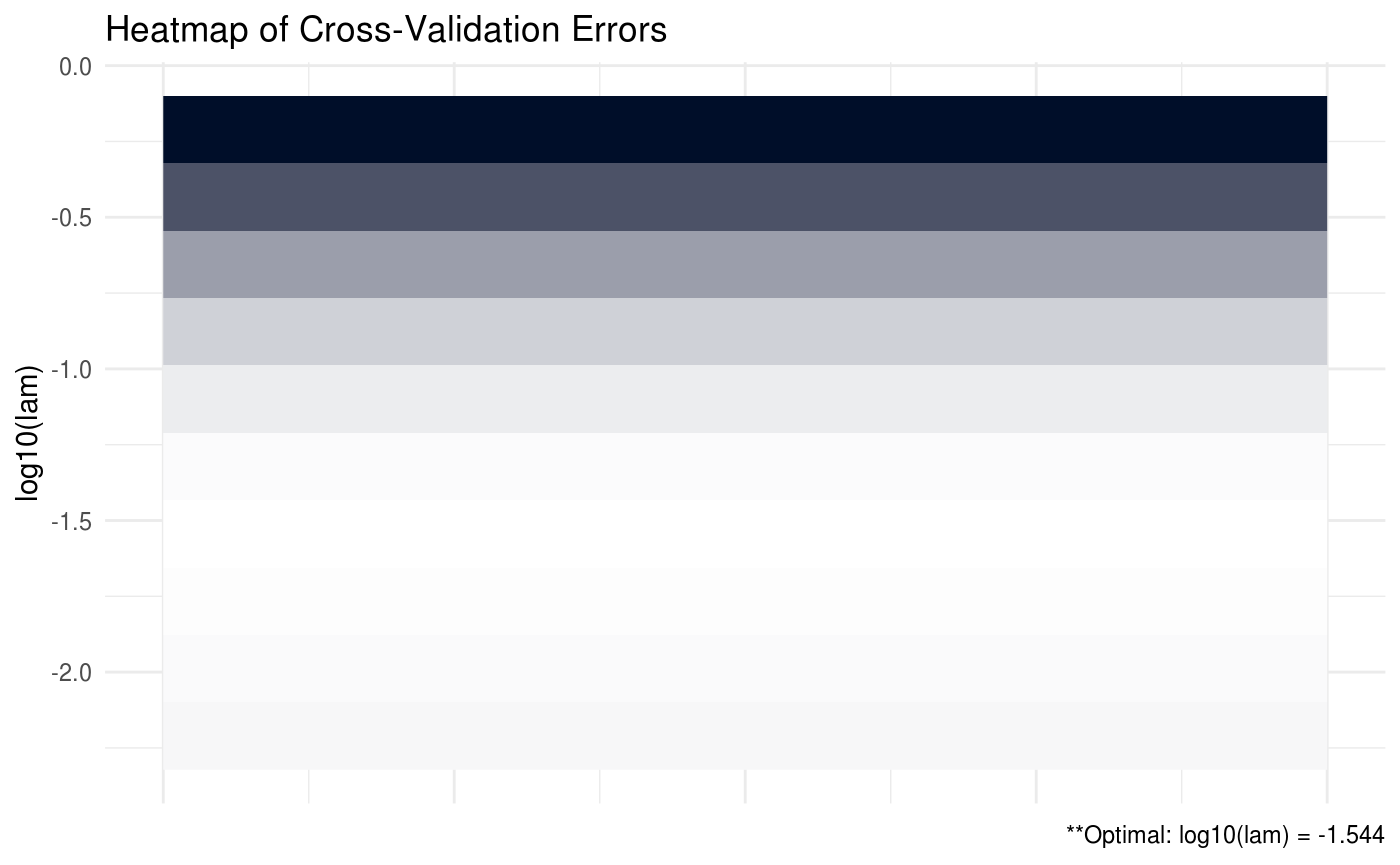
## [5,] 0.18709 0.00000 -0.00113 -1.17086 1.86326GLASSOO also has the capability to provide plots for the cross validation errors. This allows the user to analyze and select the appropriate tuning parameters.
In the heatmap plot below, the more bright (white) areas of the heat map correspond to a better tuning parameter selection.
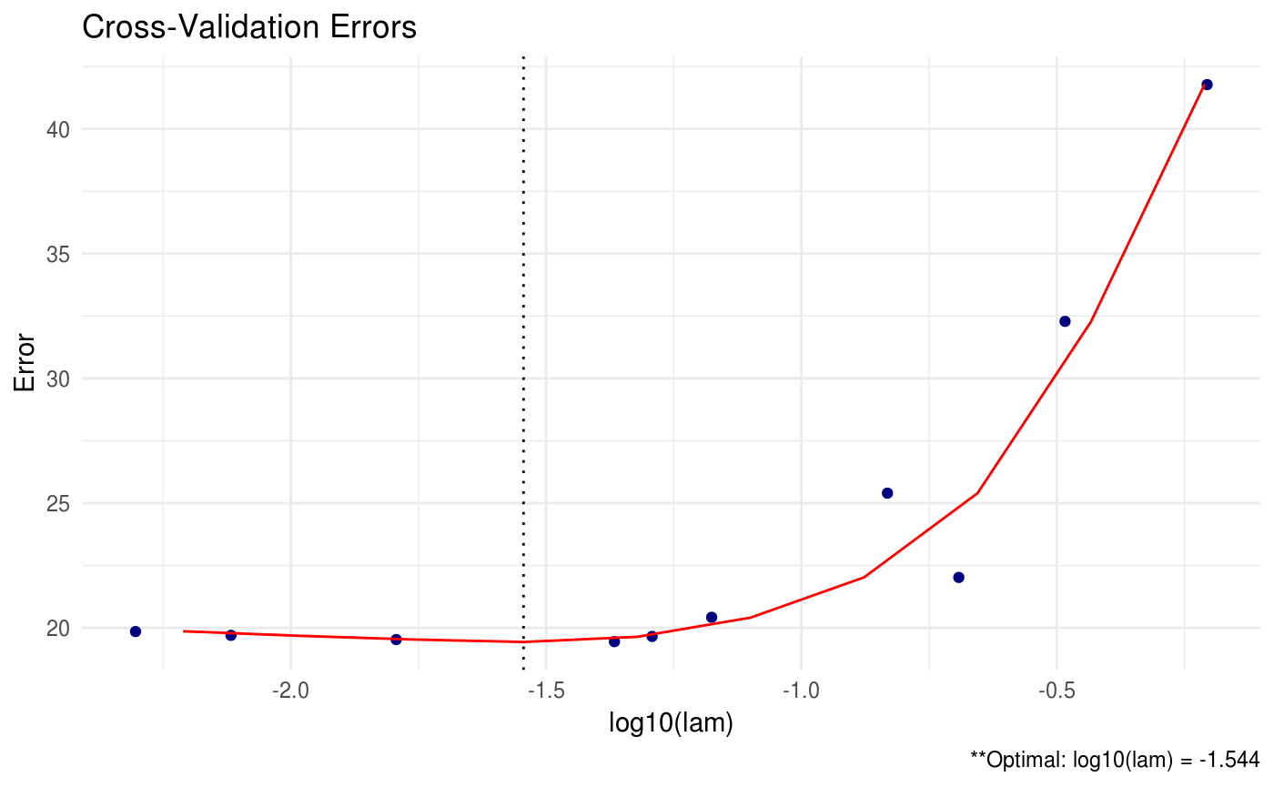
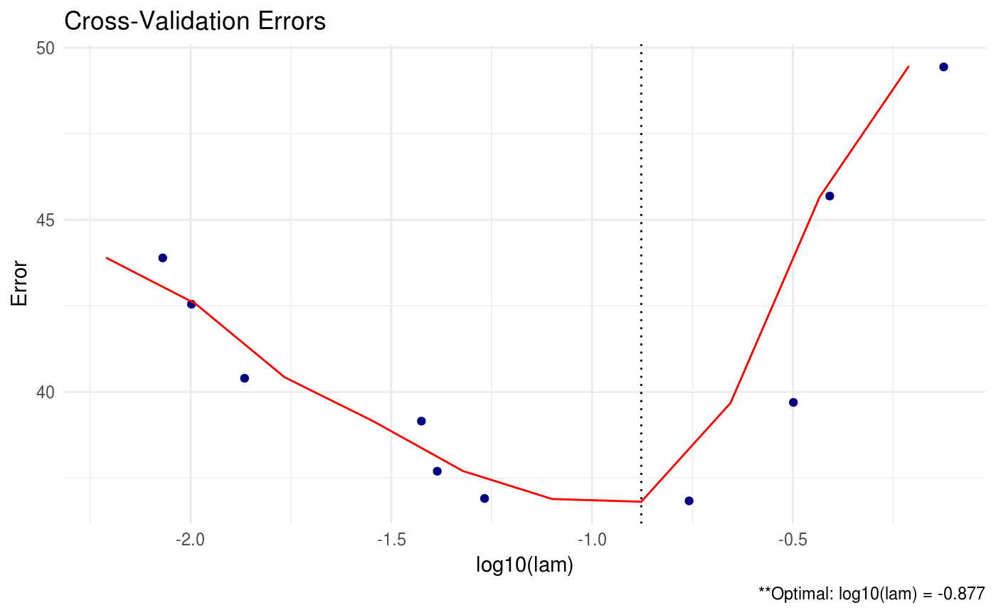
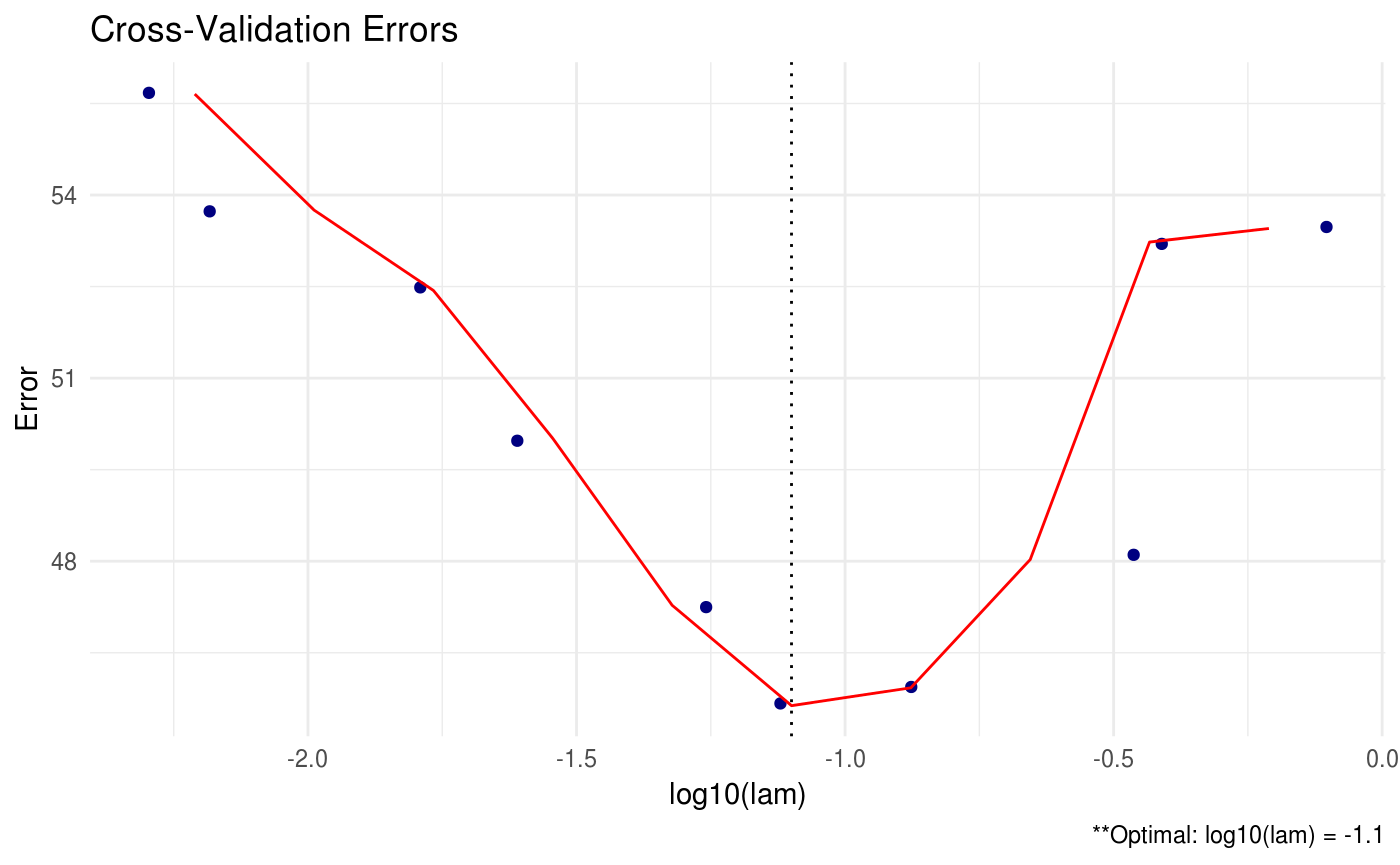
We can also produce a line graph of the cross validation errors:
GLASSOO contains a number of different criteria for selecting the optimal tuning parameters during cross validation. The package default is to choose the tuning parameters that maximize the log-likelihood (crit.cv = loglik). Other options include AIC and BIC.
This allows the user to select appropriate tuning parameters under various decision criteria. We also have the option to print all of the estimated precision matrices for each tuning parameter combination using the path option. This option should be used with extreme care when the dimension and sample size is large – you may run into memory issues.
# keep all estimates using path
CV = GLASSO(X, path = TRUE, trace = "none")

# print only first three objects
CV$Path[,,1:3]
## , , 1
##
## [,1] [,2] [,3] [,4] [,5]
## [1,] 2.27655455 -1.4550800 0.11832226 -0.03363237 0.22608180
## [2,] -1.45507998 3.1160332 -1.54994719 -0.14471035 0.14452871
## [3,] 0.11832226 -1.5499472 3.09654525 -1.22833336 -0.08600723
## [4,] -0.03363237 -0.1447104 -1.22833336 2.69276468 -1.31850681
## [5,] 0.22608180 0.1445287 -0.08600723 -1.31850681 2.00327090
##
## , , 2
##
## [,1] [,2] [,3] [,4] [,5]
## [1,] 2.2459225475 -1.3976353 0.05516907 -0.0006411027 0.21438684
## [2,] -1.3976352520 3.0205143 -1.47223070 -0.1450769526 0.11690926
## [3,] 0.0551690669 -1.4722307 3.03659758 -1.2149135832 -0.07082947
## [4,] -0.0006411027 -0.1450770 -1.21491358 2.6464667250 -1.28533809
## [5,] 0.2143868437 0.1169093 -0.07082947 -1.2853380899 1.97235485
##
## , , 3
##
## [,1] [,2] [,3] [,4] [,5]
## [1,] 2.2011297 -1.31904581 0.00000000 0.0000000 0.21425637
## [2,] -1.3190458 2.88783619 -1.38169725 -0.1137919 0.06181734
## [3,] 0.0000000 -1.38169725 2.94865501 -1.1948437 -0.04310247
## [4,] 0.0000000 -0.11379187 -1.19484367 2.5742716 -1.23897159
## [5,] 0.2142564 0.06181734 -0.04310247 -1.2389716 1.92899331More advanced options
A huge issue in precision matrix estimation is the computational complexity when the sample size and dimension of our data is particularly large. There are a number of built-in options in GLASSO that can be used to improve computation speed:
- Reduce the number of
lamvalues during cross validation. The default number is 10.
- Reduce the number of
Kfolds during cross validation. The default number is 5.
- Relax the convergence critera for the graphical lasso algorithm using the
tol.outoption. The default for each is 1e-4.
- Adjust the maximum number of iterations. The default is 1e4.
- We can also opt to run our cross validation procedure in parallel. The user should check how many cores are on their system before using this option.